The theme of the following four sections of the blog is that innovation, not price competition, is the basis for understanding economic growth, competition, and analysis.
Basic Concepts and Theory
Market Behavior and StructureMarket
Dynamics and Information: How Markets Work
Economic Theory and Markets
Corporate Strategies
There is beginning a historic change in future populations and their demographics. This will interact with other variables and have a serious, maybe profound, effect on future economic growth.
Demographics and Economics
China
Geopolitics and the Global Economy
American Economic History
Management
The world seems to be in the midst of radical political and social change. Where are we going? Can studying past periods and countries facing disrupting change help us navigate our times? Maybe.
History
American History
World War I: The Beginning of the 20th Century
The Roman Republic and America – Differences and Some Possible Parallels
Economic and Fiscal Policy
Financial Markets and Investment Strategies
Foreign Exchange Markets The United States American Foreign Policy and International Relations Geopolitics and the Global Economy Geopolitics of Oil and Natural Gas
Visionaries
Humor, Satire, WhimsyI Heard the News Today Higher Education
Examples of Bilateral Oligopoly MARKET DYNAMICS AND INFORMATION: HOW MARKETS WORK This group of posts emphasize the dynamics of economic growth and development, They highlight the role of information in the functioning of modern markets.
John von Neumann, Alan Turing, and Claude Shannon (creator of information theory) knew each other, knew of each other’s work, and discussed their ideas with each other. John von Neumann Sees the Future
(2010)GEOPOLITICS OF OIL AND NATURAL GASThe geopolitics of oil will continue to remain important until the switch to substitute renewable resources and EVs. Energy and Geopolitics I: The United States(2015)
Surprisingly, some of the comments in the following essay may be somewhat relevant to the United States, more dependent on fracked oil and lagging in innovating substitutes that drive future economic growth and development.
If you don’t know the background of this complicated story, you might want to first read a shorter version that introduces some of the key factors explaining the Crash and the Depression. See,
Before reading this essay, I strongly recommend you see the PBS video on YouTube. Type in Stock Market Crash 1929. Look for US – The Crash of 1929 (PBS), ALLHISTORIES – PLAYLIST.
Documentary broken into 6 parts to show commercials. Or buy the video on Amazon Prime. Great documentary with wonderful photos, videos, and scenes from movies of the 1920s and the crash. Shows what a crazy time it was.
The video is also a great introduction to Andrew Ross Sorkin, 1929: Inside the Greatest Crash in Wall Street History – and How It Shattered a Nation. This book concentrates on the roles played by a small number of key men; the video also focuses on these men and their social environment.
The following quote that introduces this essay is from Mr. Sorkin’s book.
The stock market is a mirror whose function it is to provide an image of the underlying or fundamental situation. Cause and effect run from the economy to the stock market, never the reverse. An unstable economy can be disturbed by all kinds of incidents that on the surface appear extraneous.
Jesse Livermore
Famous stock market speculator
INTRODUCTION
The usual reason given for the Great Depression – the stock market crash in October 1929 and the later collapse of the banking system – does not tell the whole story. Available economic data (there were no national income accounts in 1929) indicate that a recession had already begun before the stock market crash. The crash of October and November of 1929 was a catalyst that made the recession worse, but the partial stock market recovery in early 1930 did not end the recession. Industrial production continued to fall quickly and unemployment rose rapidly in 1930. As the economy sunk lower into depression and unemployment reached catastrophic heights, continuing farm and businesses failures over the next two years wiped out thousands of small rural banks and threatened total financial collapse in early 1933.
For a fuller explanation, we have to go back to the 1920s to see additional reasons for the stock market crash of 1929 and the rapid decline in output at the beginning of the Great Depression. We have to look at the international financial situation and how it contributed to America’s depression, including the attempt after World War I to reestablish the pre-war gold standard.
Economic Growth in the 1920s: Industrial Production and the Real Economy
There was a spectacular increase in industrial production starting in the 1870s and continuing into the 1920s. The 1920s were a decade of economic growth and development. The large increase in manufacturing output in this decade was driven by innovation in new and greatly expanding industries and companies.
The structure of the economy changed in the 1920s, with consequences for the stock market and financial markets in general. Industrial production, especially of large corporations, were a larger and more important part of the total economy. In contrast, agriculture stagnated in the 1920s. In 1920, agriculture accounted for 18% of Gross Domestic Product (GDP, a measure of total output); by 1929, agriculture’s share had fallen to 12%.
The foundations of the new economic structure were corporations building large-scale manufacturing plants with electricity replacing steam as the power source, new steel machinery, lower transportation and information costs, increased productivity (output per worker), and lower unit cost.
The drivers of economic growth were the new and developing technologies.
consumer durables, especially autos, electrical appliances, and radios.
electricity utilities.
mass communication (phones) and entertainment (radios, phonographs, movies).
mass-produced consumer nondurables such cosmetics, toiletries, processed food, and cigarettes.
Steel was the basis for the new auto industry, modern machinery, and skyscrapers. The amount of railroad track increased eight times from 1870. Thousands of miles of paved roads were built in the 1920s. The telephone system became ubiquitous and transcontinental with an increase in transmission bandwidth.
The 1920s was a decade of economic growth and development but it was uneven. It began with a severe deflationary (prices going down) recession as the economy adjusted from the World War I wartime economy to a peacetime economy. Economic growth began in 1922. The stock market grew rapidly in 1922 and 1923, and kept growing until late in 1929. But in 1927 and 1928, the economy hardly grew at all. Growth for the two years was about 1% per year. One reason for the 1927 stagnation was the bursting of the Florida land boom bubble (in video). This bubble showed large numbers were willing to speculate on something they knew nothing about but thought they would get rich quick. (See Marx Brothers movie Cocoanuts. Groucho was wiped out by the market crash. The movie, ironically, was released in 1929.)
Another reason was the total shutdown of Ford in 1927. Henry Ford finally scrapped the Model T and retooled his plants to produce an entirely new auto. He laid off 60,000 workers. There were spillover effects on other major industries such as steel, tires, and glass. Full production was not reached until 1929.
But strong economic growth returned in 1929. The annual growth rate was 6%. Industrial output grew faster. This strong growth was led by increased production of autos, radios, electrical appliances, and new consumer goods.
The economic expansion of 1921-1929 was based on the development of new technologies like radio and the expansion and sales of consumer durables like autos. The urban and regional buildout of the electric grid (and lower rates) led to demand for new electrical appliances and large productivity gains in mass production. Car ownership increased from about 7 million in 1919 to 27 million in 1929, on average about one car per household. This created demand for complementary products and services such as steel alloys, refined oil products, gas stations and mechanics, paved roads, and motels.
Radio (RCA) and others went from selling hobby kits in 1919 to sales of $60 million in 1922 to sales of $426 million in 1929. (Figures on car and radio sales are from digital history.uh.edu, “The Consumer Economy and Mass Entertainment.”)
Auto production was an important part of the industrial economy in the years leading up to the stock market crash. The auto industry produced approximately 4 million cars in 1926, fell to 3.1 million in 1927 because of the Ford shutdown, recovered in 1928, and reached a record 5.4 million in 1929.
Sales of these products was greatly enhanced by a large increase in consumer credit. General Motors started its own credit operation in 1919. Sears quickly followed by offering installment plans on appliances and other products. (Singer Sewing Machine Company started an installment payment plan in the 1800s.) Hundreds of new consumer credit companies were started in the 1920s.
New industries were created or greatly expanded in new types of passive entertainment (movies and phonographs) and mass consumption products like packaged food, cigarettes, toiletries, and cosmetics. Marketing and advertising encouraged consumption.
Economic growth and industrial production helped to create and expand a new middle class including managers, engineers, accountants, and lawyers. So did the expansion of the financial sector. This middle class had rising income and savings. They provided many of the new speculators in stocks in the 1920s.
Industrial Corporations and Stock Markets
Starting in the late 1800s, new and rapidly-growing industrial corporations needed large amounts of investment and expansion capital, far more than what they could generate from internal cash flow. Capital was needed to take advantage of scalability (economies of scale).
The stock market, and the financial sector in general, had become increasingly important to the American economy during the 60 years leading up to the crash of 1929. In the 1920s, the financial sector doubled as a percent of the national economy. Its growth paralleled the financial requirements of new and growing companies. New, capital-intensive, large, and growing corporations needed investment capital far in excess of what company founders and rich backers could provide. The solution was the creation of the publicly financed, limited liability corporation. The canals starting in the 1820s, the railroads starting in the 1830s and then the industrial corporations starting in the 1870s issued stocks and bonds to the public to finance their capital requirements. In an expanding economy, investors could expect to collect dividends and watch their stocks appreciate in price.
Equity capital (stock) had the advantage over bonds that the corporation was not obligated to buy back the securities. Or pay a fixed amount of interest. But investors were “locked-in.” This might have limited the attraction of equity investment except that investors in public companies could exit by selling their stock to others in “secondary” markets like the New York Stock Exchange (NYSE).
So large companies and stock exchanges were connected, complementary, and grew together.
The Stock Market Crash of 1929
In the 1920s, the “stock market” meant the New York Stock Exchange. This is where the shares of most large companies were bought and sold.
The New York Stock Exchange was a private company, owned by its members. Until the 1920s, most stock traders were full-time professionals. There were no rules or laws. Traders lied, cheated, and deceived among themselves. In the 1920s, they could now also do this to naïve small investors. They viewed small investors as sheep to be shorn.
In 1929, there were 1,334 companies whose stock was traded on the New York Stock Exchange. This was a tiny percent of all the farms and businesses in America. But these were most of America’s largest companies. They accounted for much of the economic growth in the 1920s.
Many of the companies on the NYSE dominated their industries and markets. They had exhibited large increases in sales and profits over time, which led to high expectations for rapid future growth in company sales and profits.
The impression that “everyone” was playing the stock market is an exaggeration. By 1929, fewer than one out of ten families had money in the market. They were about half of all families with financial assets. Stocks, like consumer durables, were often bought on credit, or “margin,” by some of the speculators. About half of small investors bought on margin. Typically, the investors put up 10 – 20% of the value of the stock and borrowed the other 80 – 90% from the broker. The stock was collateral for the loan. The broker, in turn, borrowed the money from banks and other institutions with spare cash. Brokers’ loans (also known as “call money” because they were overnight loans and could be “called” in one day) increased about $1 billion in 1920 to $4.4 billion in early 1928 to $8.5 billion in October 1929.
About 80% of the brokers loans came from sources outside the banking system, including overseas, so Fed pressure on member banks not to make call loans had little effect. The loans seemed safe as long as the stock collateral increased in value. Interest rates were higher than alternative short-term loans.
Small investors leveraged their bets even more by using margin to buy stock in new investment trusts. Investment trusts were similar to today’s mutual funds except they were also leveraged – selling both shares to investors and floating bonds. Then leveraged investment trusts bought shares in other leveraged investment trusts. Alas, leverage also worked on the downside; owners of shares in investment trusts were wiped out even when the shares of the underlying companies still had some value.
The speculative bubble, when stock prices rose much faster than earnings and earnings per share, began in March 1928. As measured by the Dow Jones Industrial Average, stock prices doubled and reached an all-time high the day after Labor Day, September 3, 1929. The Dow Jones index went from 200 to 390. The total value of stocks had gone from $25 billion to over $50 billion, in an economy of $100 billion.
By 1929, investors had high expectations about the percent increase in stock prices. Based on the yearly increases from the beginning of 1928 to September 29, conservative investors who paid cash and bought a diversified portfolio of stock like the Dow Jones index, expected returns of 50%/year. If they bought stock on 20% margin, they expected to make over 200% a year; on 10% margin, over 400% a year.
Investors who bought leveraged investment instruments like investment trusts with margin expected an even higher yearly return.
Speculators bet on companies like Radio (RCA). RCA was up 500% since beginning of 1928.
There were also short-term bets based on rumors about big pools of capital going into a stock. Often a big speculative pool started buying a stock. They paid for a lot of publicity, including bribing financial journalists to hype their stock. As more small speculators piled in, the pool started selling. Small investors were left holding a bag of stocks with rapidly falling prices. (See video)
While corporate profits were going up, stock prices were going up even faster. This led to record high stock price/earnings per share (P/E) ratios. This was viewed as an indication of rising confidence that the market would continue to go up. But the market’s P/E ratio would have to continue to rise if the market continued to go up at 50% a year.
The Dow Jones index reached its high on September 3, 1929. The market slowly declined for a few weeks and then crashed at the end of October. The market was down nearly 13% on Monday, October 28. The climax, in massive volume, was the next day, October 29 (Black Tuesday), when the market fell 12%. The total drop from its September high to the end of October was 40%.
By the end of November 1929, the stock market had fallen 50% and had wiped out all of the speculative gains since early 1928. In early 1930, it reversed direction and regained 40% of its 1929 losses. Volume was high. But in April commodity prices started to fall again. Industrial production continued to decline all through 1930. Unemployment rose quickly. The market turned down again. By late 1930, the stock market had fallen below its November 1929 lows.
The entry of large “pools” of outside speculative capital and small investors into the stock market was one reason for the bubble. This was something new; until the 1920s, stock market participation was an insider’s game of professional speculators. But now insiders and investment managers of outside capital could manipulate stock prices at the expense of small investors.
Partners of the largest investment banks, market analysts, government officials, congressional committee hearings, and Fed officials had private doubts or warned the public of the dangers of the “over-priced” market. But their messages were drowned out by reassuring and optimistic statements of market boosters like Charlie Mitchell of National City Bank who had done much to encourage margin buying by new small investors. Negative comments were ignored by speculators caught up in the frenzy. Instead, they listened to advisors like the foremost astrologer of the day, who predicted the market would go up forever. Presumably to the stars (see video).
The stock market crash of October 1929 did not come as a surprise to everyone. Some of the biggest speculators like Jesse Livormore and investment bankers like some of the partners at J.P. Morgan sold their positions before the crash. Livormore shorted the market (bet it would go down); when he came home on the worse day of the crash, he told his wife he had made more money that day than any other day in over 20 years of speculating.
Before World War I, about a half a million shares were traded on a typical day. In 1928 and 1929, volume was rising rapidly, averaging about five million shares a day. On October 29, volume hit an all-time high of 16 million shares. Stock prices were on average six times higher than earlier in the 1920s, so that the combination of more speculators, and more of them acting like short-term traders, led to a huge increase in the dollar value of the stock market.
Investors’ and large speculators’ margin of 10%-20% was wiped out in just two days, October 28 and October 29. Margin calls for more cash went out; if not provided immediately, the broker tried to sell the underlying stock, increasing supply. Banks and other providers called their loans. All this led to a cascade of hitting stop-loss orders and more margin calls. In the fall of 1929, about $2 billion of brokers’ loans were pulled out or wiped out.
Large investment pools, like the one controlled by Billy Durant (who put together General Motors and then drove it into bankruptcy), speculated on margin and also lost heavily in the stock market crash. When stock prices fell, they doubled down – buying more stock – only to see their losses increase. Durant personally lost $18 million. One of the richest men in America (on paper) in 1929, he never recovered and finally declared personal bankruptcy in 1936. Jesse Livermore, probably the most successful individual speculator in the 1920s, made a series of bad bets in the 1930s and committed suicide in 1940.
The large, sharp decline in the stock market had an immediately negative impact on aggregate (total) demand, especially demand for consumer durables usually bought on credit and luxury goods and services. Expectations of rising personal wealth and a higher standard of living from rising stock prices were shattered.
After the bubble burst, the New York Fed reacted quickly. In the six months after the crash, the New York Fed injected $500 million of liquidity into the banking system. It cut its rediscount (loan) rate to banks from 6.0% to 2.5%. New York banks, in response, took over $1 billion in brokers’ loans. No major New York bank failed. The market rallied in the first half of 1930. It appeared the crash had been contained. It wasn’t.
It was not because of:
the weaknesses in the American economy, especially the farm sector.
the fragile international financial system, based on the gold standard, constructed after World War I.
the fragmented American banking system watched over by passive regional Fed banks.
the rising importance of the financial sector, and how it interacted with the real economy.
The Farm Economy
The period from the mid-1890s to 1918 has been called the “Golden Age of American Agriculture.” Expansion into new areas, rising demand from American and European urban areas and industry, rising prices, and World War I (large food exports to England) all led to prosperity for the farming sector.
In addition to the usual seasonal loans, farmers went deeper in debt to expand acreage (the average size farm increased) and buy large amounts of new equipment, including tractors, to increase productivity and lower unit cost. They also bought new cars (mostly Model T Fords) with borrowed money. During this period, thousands of new banks were started in rural areas to finance this expansion.
Agriculture was still a major part of the economy. In 1920, the farm population was 30% of the total U.S. population. Almost 50% of Americans lived on the farm or in towns with fewer than 2.500 people, many of them in rural areas dependent on agriculture.
The farm economy went into recession during the price deflation after World War I and remained stagnant during the 1920s. Farm prices fell in half after World War I and then slowly declined as American farmers lost their European markets. European demand fell because of the violence, chaos, and disruption caused by the war.
Attempts by the Hoover Administration to stabilize farm prices through purchasing surpluses failed. In 1930, the market price of wheat fell in half. Further large decreases after 1930 in farm prices and the “Dust Bowl” collapsed the agricultural sector, farmers defaulted on loans at a rate of 1,000 a day, resulting in the bankruptcy of thousands of small, rural banks.
Eight rural states set up deposit insurance programs before and during the 1920s. All failed by 1929. Depositors (savers) were ruined along with the banks since there was no federal deposit insurance before 1933.
Large industrial corporations created and dominated markets. The raising of large amounts of financial capital fueled buying the more efficient capital equipment and industrial expansion. Large industrial companies employed factory workers, office workers and new types of professionals like engineers, chemists, accountants, and managers. Combined with the stagnation of the rural sector, America became an urban, industrialized society.
Investors in corporate stock did not always understand why stock prices were rising. Mass production processors and assemblers had high fixed costs in capital equipment. Some of it was financed with debt, creating financial leverage. Companies had to run at a high percent of rated capacity to make a profit. A small increase in sales (output) resulted in a leveraged increase in profit. Stock prices rose with rising profits; expectations of future increases in profits led to higher stock price to earnings (P/E) ratios, also increasing stock prices. This worked in reverse, starting in late 1929. Decreases in sales led to leveraged decreases in profits. Stock prices fell. Expectations of further decreases in profits lowered P/E ratios causing even lower stock prices.
Real incomes rose in the 1920s. But, like today, income and especially wealth was concentrated.
One estimate is that about one-third of all income was going to the top 5%. Sales of luxury goods and services soared. In contrast, farm families experienced a fall in total real income.
Demand for many consumer durables was partly paid for with a large increase in consumer debt called installment loans (buy now, pay later). As an expanding urban middle class and working class financed their rising standards of living partly through increased borrowing, household debt rose faster than income. By 1929, about 60% of cars and 75% of all radios were bought on credit. (A top-of-the-line radio cost as much as the average cost of a car!) Total consumer debt doubled in just four years, going from $1.4 billion in 1925 to $3.0 billion in 1929. Hundreds of new banks and finance companies were started to provide consumer credit.
Home ownership financed by new forms of mortgage debt rose rapidly. Mortgage debt rose over eight times from 1920 to 1929. Hundreds of new “saving” banks were started to supply mortgages.
Household balance sheets were leveraged with consumer debt and mortgages backed by illiquid assets as collateral that quickly lost market value starting in the fall of 1929. Even as savings were being wiped out, families still had to make installment and mortgage payments.
By October 1929, the economy was already in recession. Railroad car loadings and steel production had been falling since summer. The Fed’s Index of Industrial Production was also declining. Auto inventories were rising. But a general recession wasn’t recognized and declared until late in 1929. These numbers had little influence on analysts or investors.
1930
The recession was sudden and severe. Industrial production fell about 5% in October and another 5% in November. The contraction continued into 1930; industrial production fell another 30%. Unemployment doubled, from about 1.5 million (3% of the workforce) in the summer of 1929 to about 3 million (6%) in the spring of 1930, and then rose to about 5 million (10%) at the end of 1930. At least 25% of American families – a higher percent of non-farm families – were hit by unemployment sometime before the end of 1930. About half of the Great Depression’s total decrease in industrial production and about half of the increase in unemployment had already occurred by late 1930. Families experiencing unemployment couldn’t meet loan payments. (Most urban families were one-income families. Also, there wasn’t unemployment benefits like today.)
In 1930, farmers were hit with lower prices, the Dust Bowl (huge dust clouds), loss of deposits in local failed banks, and inability to make loan payments on equipment. Farmers started to lose their farms; banks foreclosed on about 100,000 farms in 1930. (See the movie and/or read the book about this – The Grapes of Wrath.) The Dust Bowl continued until 1940, helping to wipe out many more farmers (see PBS video on the Dust Bowl; the dust clouds are unbelievable).
Demand for consumer durables was especially hard hit. Car sales were 5.4 million in 1929, falling about one-third to 3.4 million in 1930. (At the bottom of the depression, auto production would fall by 90%.) Sales went from $3.5 billion in 1929 to $0.8 billion in 1932. Repossessed and used cars glutted the market. (Good for my grandfather; he bought a used truck in the 1930s for $30 to start a small business. The seller had to teach him how to drive.)
AFTER 1930 – A QUICK SUMMARYAs the Great Depression got worse, stock prices kept going down, about 5,000 more banks went under wiping out depositors, unemployment rose to catastrophic heights, families couldn’t meet loan payments and lost their houses and cars.Eventually, almost half of all mortgages were in default.When the worse was over, real GDP fell by about 25% and nominal GDP went from about $100 billion in 1929 to about $50 billion in 1932. In 1929, corporations made total profits of about $10 billion; in 1932, they lost about $3 billion. Business investment disappeared.The depression and consequent disappearance of corporate profits (earnings) had consequences for stock prices. Using valuation metrics like price/earnings (P/E) ratios, there was no support level, no bottom, for stock prices. The other support for stock prices – dividends – also fell drastically as profits disappeared. Trading volume fell, from an average around 10 million shares per day in October 1929 to around a half a million shares per day in 1932.By 1932, market indexes had fallen 80-90% from October 1929.The negative reinforcing feedback effects between the real economy and the financial sector created the Great Depression. Again, the size of the total economy was about $100 billion in 1929. Between 1929 and 1932, stocks (and stockholders) lost about $30-$40 billion in value. Total bank credit fell $20 billion.
WAGES AND PRICES
Wages and prices acted differently at the beginning of the Great Depression compared to earlier recessions. The Consumer Price Index (CPI) went down only 2.6% in 1930. Nominal (current dollar or money) wages in the large industrial corporations, and other large companies, stayed virtually constant in 1930. Industrial prices also did not decline. Instead, large manufacturing firms laid off employees and cut production, watching sales and profits plummet. Investment stopped, hurting the capital goods sector. The question all this raises is: Why didn’t large companies quickly cut wage and prices, as in prior recessions?In a series of conferences in November and December 1929, President Herbert Hoover urged the leaders of the largest companies not to cut wages. Many corporate presidents agreed, including the presidents of General Motors, Ford, General Electric, Westinghouse, Standard Oil, U.S. Steel, Du Pont, Firestone, and Goodrich. The idea was that by not cutting the wages, and therefore income, of their workers, they were helping to limit the fall in overall (aggregate) demand. Keeping wages and thus prices high probably contributed to the large decreases in demand for consumer durables. As demand and output fell, these companies laid off workers, contributing to the rapid increase in unemployment. It was only in late 1930 and 1931 that large companies began cutting wages.In 1933, President Franklin Roosevelt had Congress pass the National Recovery Act (NRA), an economy-wide, mandatory version of President Hoover’s voluntary program.
FINANCING ECONOMIC GROWTH AND DEVELOPMENT IN THE 1920SThe financial sector as a whole was a growing part of the economy in the 1920s. Finance doubled as a share of GDP with most of the growth coming in the second half.The raising of large amounts of financial capital fueled the economic expansion, not just on the supply side but also on the demand side.An expanding urban middle class financed its rising standard of living partly through increased borrowing; household debt rose faster than income. In addition, mortgage debt rose rapidly. Household balance sheets were leveraged with debt backed by illiquid assets that quickly lost market value starting in the fall of 1929.The purchase of consumer durables such as autos, radios (some cost as much as cars), furniture, and some electrical appliances was usually financed with debt, often with money borrowed at the new consumer finance companies. Miss one payment and the product was repossessed. One of the largest banks that specialized in car loans, controlled by Henry Ford’s son Edsel, went under.
THE AMERICAN BANKING SYSTEM AND THE FED
At the beginning of 1929, the United States had 25,000 banks. Most, about two-thirds, were outside the Federal Reserve System (the Fed). States and the federal government had passed laws to protect local banks from competition from larger banks by limiting the geographical reach of banks. The small rural banks depended on the health of the local farm economy. It should have been an alarm bell as thousands went under in the decade before the crash.Between 1929 and 1933, the U.S. banking system – unregulated, fragmented, without deposit insurance – went through waves of bankruptcies as farmers, businesses, and consumers defaulted. In the two years 1929 and 1930, about 10% in of the total number of banks failed. About a third of all banks would disappear during the Great Depression. Depositors lost their savings. Farmers and processors could not repay loans and small, local banks went under. Solvent farmers could not get credit to produce. Urban and suburban banks started to go bankrupt as consumers, local businesses, and homeowners defaulted on loans. At the depth of the depression, half of all mortgages were in default.
Why did not the Fed save the banking system from collapse? One of the Fed’s powers was to be the “lender of last resort” to member banks. Banks in a liquidity squeeze could borrow at the rediscount window at the Fed banks. This was limited since one-third of banks were members of the Federal Reserve System. But they were the larger banks; smaller banks typically held part of their reserves at larger banks. As the economic crisis deepened, small, local banks began asking for their deposits at the larger banks. This reduced reserves at the larger banks which were not balanced by new liquidity from the Fed.
Through all this, the eleven regional Fed banks outside of New York and the governing board in Washington did virtually nothing. Controlled by local bankers and manufacturers, they did not believe it was their responsibility to save the banking system. Their governing boards limited the types of collateral they were willing to accept from borrowing banks at the discount window. They did not actively encourage local banks to apply for funds. The exception was the sixth regional located in Atlanta. They faced the first regional banking crisis and successfully contained it.
This attitude of letting the economy and its banks to go to hell was shared by Andrew Mellon, Hoover’s Secretary of the Treasury, who believed a major recession was good for the health of the economy. (He was too busy adding to his fabulous art collection by secretly and illegally buying art from the Soviet Union, which needed hard currency to finance its spying operations. These paintings, taken from the Hermitage, are now in the National Gallery collection in Washington. The spies later stole America’s atomic bomb secrets.)
By the spring of 1933, the American banking system was near total collapse. Over half the states had declared a “bank holiday,” closing all the banks in their states to see which ones could be saved. This meant that depositors could not withdraw their savings. The new Roosevelt Administration’s first act in March 1933 was to declare a national bank holiday. Roosevelt’s second act was to take the United States off the gold standard.
INTERNATIONAL ASPECTSIn the 1920s, New York had become the center of the global financial system. This was a consequence of World War I and its aftermath. During the war, England and France partly financed their war effort with substantial borrowing from New York banks. England and France could not borrow from the American government because Wilson was afraid isolationists could help defeat him for reelection in 1916. During the 1920s, Germany borrowed large sums from New York banks to restart its economy and pay war reparations to England and France.Central bankers and large investment banks spent the 1920s trying to rebuild the global financial system shattered by World War I. They saw the pre-war gold standard as a control mechanism to overcome the economic dislocation and instability caused by the war. The key, as they saw it, was to fix the value of national currencies in gold and thus, to each other. By 1929, almost all currencies, including the dollar, were on the gold standard. (In a bit of bad timing, Japan went on the gold standard in January 1930.)The gold standard depended critically on the pound sterling and London before the war, and the dollar and New York after the war. The New York Fed chairman (Benjamin Strong) worked closely with the chairman of the Bank of England (Montagu Norman) and other central bankers to coordinate policy, primarily changes in interest rates to influence currency and gold flows. Central banks and investment banks, mostly American, would also loan money to foreign governments to ease pressure on their currency. But America’s commitment to reforming the global financial system was limited. There were three major problems:1) Entente (Allies) war debts and German reparations. The Entente countries, including England and France, had borrowed over $10 billion in America to help finance the war. After the war, the Allies imposed reparations on Germany, payable mostly to England and France. These two countries relied on payments from Germany to meet the interest and principal payments on their debt to the United States. But the German economy had a hard time recovering from the war and taxing its people to raise reparation funds. Instead, Germany depended on borrowing from private banks in New York. Some of the funds would then go to London and Paris, to be cycled back to New York. Towards the end of the 1920s, more of the loans were short-term (“hot money”) rather than the usual long-term credits. The system functioned as long as American bankers were willing to lend to Germany, that is, to roll over rather than call short-term loans.
2) England went back on the gold standard in 1925 at the pre-war parity. It overvalued the pound compared to other currencies. English exports were priced out of global markets; imports were relatively cheap. As a consequence, the English economy had a hard time recovering from the war, experiencing deflationary stagnation. England ran a trade surplus before the war but a trade deficit after the war. Defending sterling’s price in gold meant high interest rates to attract foreign funds, low economic growth, deflation (with pressure on wages), and high unemployment rates.
The New York Fed often changed American interest rates to accommodate the Bank of England’s attempts to deal with England’s economic and financial problems.
3) Central bankers would change interest rates to influence cross-country capital and gold movements. But changes in interest rates also affected domestic economies. Interest rates in New York were actually lowered at the beginning of the stock market boom to encourage money flows to England. But lowered rates also reduced the cost of call money and brokers’ loans to speculators, fueling the stock market bubble.Gold was also “high-powered” money, a part of the banking system’s reserves. An influx of gold allowed a country’s banking system to created money by creating new loans. Throughout the 1920s there was a net inflow of gold into the United States. American banks could increase the amount of loans to American consumers, stock market speculators, farmers, and corporations.
Just when it seemed the global financial system was stabilizing, it started to unwind. Germany went into recession in 1928. The head of Germany’s central bank threatened to stop paying reparations. Money flowed out of Germany. American bankers stopped expanding short-term loans to Germany. The American government refused to reduce Allied war debts; England and France could not reduce debt payments to private American banks. By 1929, Germany had reduced paying war reparations and the crucial cycle of American loans to Germany, German reparation payments to England and France, and their war debt payments to American banks began to unravel. American banks were now sitting on billions of dollars of bad loans. A delegation of American bankers went to Europe to renegotiate the repayment timetable of German reparations. A slowdown in economic growth in the industrialized countries led to a large decrease in global commodity prices (inelastic demand). Countries that depended on commodity exports went into recession and were the first countries to leave the gold standard.
The U.S. economy went into recession and the stock market crashed. One consequence was that American banks started calling in German loans, deepening the German recession. There was a large and sudden increase in German unemployment. This contributed to the rise of Hitler and the Nazi Party, which received only 2.6% of the vote in 1928 but over 35% in 1930. The Nazi Party was the largest right-wing party, making it almost inevitable that Hitler would become Chancellor as conservatives tried to form an effective government to counter rising left-wing support. In office in January 1933, Hitler quickly renounced all reparations payments.
By 1931, the English government realized that England would not get out of long-term stagnation without eliminating the deflationary effects of the gold standard. England and 20 trading partners left the gold standard. The English pound sterling depreciated (went down in value) against the dollar, making America’s recovery more difficult.
THE GOLD STANDARD AND DOMESTIC POLICY
The Hoover Administration’s and the Fed’s commitment to the gold standard limited domestic policy options. Budget deficits, lower interest rates, or increasing the money supply through Fed lending to banks would have tempted foreign central banks and depositors to withdraw gold. This was one reason the Fed did not use gold as part of the monetary base to expand credit through its discount window. Another reason: the Fed might lose gold and contracted credit would also happen if Americans used dollars to buy gold. This was legal until President Roosevelt took America off the gold standard in early 1933.
The worsening recession and the gold standard led to deflation. Deflation led to the higher real cost of debt to borrowers, and then defaults as incomes and asset prices fell. The banking system weakened. Banks failures rose dramatically in 1931 and 1932. Seeing the deep recession and the weak financial sector, foreigners began pulling gold out in 1932. The Fed raised interest rates to keep the gold in the U.S. The Hoover Administration raised taxes to reduce deficits and signal “fiscal responsibility.” Again, by early 1933, the entire U.S. banking system was approaching total collapse.
THE SMOOT-HAWLEY ACT OF 1930
At the beginning of the Great Depression, Congress passed the Smoot-Hawley tariff bill of 1930 to protect farmers. Of course, everyone in Congress added their favorite worthy group of constituents who wanted protection. Tariffs went up to 60%. 1,000 economists, a rather conservative bunch in 1930, warned of the negative consequences of the bill.
The main target was Canada, America’s largest trading partner. The more anti-American party won the next Canadian election.
Anti-American boycotts of American products started in Europe. American exports to Europe and Japan fell.
England walled off its Dominion countries and colonies from American imports; France and Holland did the same with their colonies. Since imports and exports were a small percent of the American economy, about 5% in total, the Smoot-Hawley tariff bill was probably not a major cause of the Great Depression. Both imports and exports fell by about $1 billion, so the Act had little net macroeconomic effect. But, on the margin, it probably contributed somewhat to the length and depth of the Great Depression.
Tariffs and other barriers to trade reenforced America’s isolationism. To keep America out of the looming European war (on England’s and France’s side), a strong America First movement arose. Some of its members, including Charles Lindbergh and a future president of Yale, were pro-Hitler. The organization effectively disbanded in December, 1941.
A LONGER VIEW OF THE STOCK MARKET CRASH OF 1929
By the end of 1929, the Dow Jones Index was back to the beginning of 1928. It was only 17% lower than the beginning of 1929 – a year of above-average gains followed by larger losses. So any investor who bought stock for cash at the beginning of 1928 or earlier, was about even. Anyone bought stock at the beginning of 1929 was even by the end of the first quarter of 1930, before the market turned down again. Only speculators who bought stock on margin were wiped out. This included many large speculators. Of course, anyone who held their stock until the end of 1932 lost almost of the value anyway. And anyone who bought on “dips” between 1929 and 1932 lost money.
It is likely that many families who still had stock after 1929 were later forced to sell because of some combination of unemployment, lose of savings in a collapsed bank, and to meet installments on borrowings for consumption and maybe a mortgage on their home.
Anyone who bought at the top in September 1929 and held onto their shares had to wait until 1954 to break even.
Since 2000, there has been three market contractions of similar magnitude to October 1929. The last two could have led to a prolong depression. But they didn’t. The difference is that the federal government stepped in with massive fiscal stimulus and support for failing companies.
SUMMARYIt is a mistake to see the stock market as separate from the rest of the economy. It was part of the financial sector, which greatly expanded in the 1920s and became a more important part of the economy. The financial sector helped finance the economic growth and new products of the 1920s, especially demand for the new consumer durables. Gains from the stock market helped to finance the flamboyant life-style of a small percentage of consumers, symbolized when wealthy Americans on luxury trans-Atlantic steamers could radio their brokers in New York with stock orders. The boom in buying consumer durables and housing was made possible by the expansion of consumer loans and home mortgages. Increases in consumption and consumer loans were tied together. In contrast, small local banks were tied to the stagnant, leveraged agricultural sector. Although the bottom of the Great Depression came over three years after the start, over half the fall in output and real income occurred in the first year, by the end of 1930. This was a large and rapid decline. The stock market crash was a catalyst; it accelerated the decline in income, wealth and the demand for goods and services through feedback effects between the financial sector and the real economy.The stock market crash of 1929 was not the only reason for the depression. Many of the systemic risks were due to global and domestic problems caused by the First World War and its aftermath. There were continuous feedback effects between the real sector and the financial sector. What changed was the size and importance of the American financial sector – as an international lender, as a raiser of capital, as a provider of household credit, as a seller of financial instruments.
The continuous feedback effects also help explain why the depression lasted so long and was so deep. Waves of bank failures, loss of savings and assets, lack of the Fed’s responsibility as “lender of last resort” all contributed to lengthening the depression and making the recovery difficult
Many of the government recovery programs of the Hoover Administration and the early Roosevelt Administration were substitutes for a financial sector that had ceased to function.
The American economy in the 1920s became not only larger but also more complex. There were more “fault lines.” Recent studies of “complex adaptive systems” indicate they can go from seemingly stable to unstable very quickly. New potential fault lines were added in the 1920s – stock market speculation, agricultural stagnation and debt, consumer durables bought with loans, and America’s involvement in international finance.
The structure (including rules and lack of rules) of the financial sector when the crisis hit was important. The banking structure and much of the rest of the financial markets had not adjusted to the economic changes of the 1920s. Fragmented domestic banking, the gold standard, lack of information and analysis, absence of oversight, and widespread manipulation and fraud all contributed to a financial sector that was ill-prepared to handle the stresses beginning in 1929. Changing the rules – increasing the confidence of depositors, borrowers and investors – was an important part of the New Deal.The depression was made worse by the antiquated mentalities of those in power. They were faced with the instabilities and dislocations of an international financial system radically changed by World War I. Their response was to revert back to the rigidity and deflationary pressure of the gold standard. American officials and the three Republican presidents in the 1920srefused to decrease Allied war debt, a necessary condition to stabilize the international financial system. In America, an increasingly industrialized, mass consumption economy fueled by financial capital and consumer debt depended on a fragmented banking system of small, local banks designed for a decentralized agrarian economy. Fed and government officials strongly believed in market competition and laissez-faire, which was ill-suited to an economy dominated by large, mass production corporations and a greatly expanded financial sector.
CONCLUSION
The real economy was growing rapidly, probably around 6% in 1929. This growth rate was unsustainable. Part of it was because of pent-up demand for autos; many consumers had waited for Ford to get back to full production. There was a big increase in the purchase of autos and other consumer durables during this period. A high percent of consumer durables were bought on credit.Rising domestic optimism was behind the big increases in both output and the stock market. Employment levels were high. This optimism is hard to quantify but it was pervasive outside of some rural districts. (See video)Recessions start with an unexpected shock. They are often outside of economic models used at the time of the shock. In 1929, the stock market decline was mostly independent of the real economy recession. In 1930, stock market recovered 40% in first quarter, indicating investors believed the decline was a “correction” and stock prices were cheap. But the real economy continued its rapid deterioration. When recognized, investors realized their optimism was misplaced and the stock market turned down again. The recession of 1930 does not show up in financial figures except for the stock market and more than the usual number of small banks failing. As the buying of consumer durables and other mass-produced consumer products declined, profits fell. Investment in manufacturing declined, as the reason for increasing capacity disappeared. The government did not make up any of the loss of income in 1930 through welfare programs or fiscal deficits. (Even during the 1930s, Roosevelt’s budget deficits were much smaller than the decline in private incomes and corporate investment. A misguided policy to balance the budget in 1937 led to a severe recession that wiped much of the output and employment gains of the prior four years.)The structure of the economy had fundamentally changed since the last depression that occurred in the 1890s. New economic and financial fault lines appeared in both rural and industrial America. The situation was made more dangerous as the global economy struggled to recover from World War I and its chaotic aftermath. Only the New York Fed and large New York banks worried about international instability and its possible consequences. Eventualy, all Americans would become aware of the consequences of post-WWI overseas problems, the stock market crash of 1929, and the beginning of the Great Depression in 1930. On December 7, 1941.
======================================================The best introduction to the 1920s and the stock market crash is Frederick Lewis Allen, Only Yesterday; An Informal History of the 1920’s. This is a wonderful popular history of the 1920s and the crash. It shows how the economic, social, and psychological changes in the 1920s contributed to the speculative frenzy in the stock market. Allen lived through it all. You can skip some of the chapters the first time through; for example, skip Chapters III, VI, IX, And X.If all of this seems complicated and confusing (it is), you might want to see a summary:
The Congressional Budget Office (CBO) made their latest projection in January, 2025. The projected deficit in fiscal year 2025 will be around $1.8 trillion, the difference between about $5.2 trillion in revenue and $7.0 trillion in expenses. Interest on the national debt this year will be around $950 billion, over twice the interest expense in the fiscal year 2021 budget and equal to the defense budget. By 2035, the CBO expects the yearly budget deficit to increase to $2.7 trillion.
Interest expense this year passed budgeted outlays for the military. It is about equal to Medicare, and also to total non-defense discretionary spending.
Leaving aside Social Security and Medicare, interest expense is about 20% of total budget outlays. Interest expense is about half the budget deficit.
The $1.8 trillion budget deficit is 6-7% of total GDP, or approximately 10% of consumer spending. Adding the $1 trillion trade deficit, which is 3-4% of GDP, then a total of $3 trillion, or 10% of GDP, is being financed by these two deficits.
SOME BASIC DEFINITIONS AND A LITTLE DETAIL
Some basic definitions for people in government suffering from political amnesia:
Deficit. The difference between the federal government’s spending and its revenue in one fiscal year. The fiscal year starts on October 1. So fiscal year (FY) 2025 started on October 1, 2024. All years in this post are fiscal years. You know right away this is going to be confusing.
Debt. Short for national debt or federal debt. The sum total of all past government yearly deficits minus yearly surpluses.
PROJECTED NATIONAL DEBT
As of June 9, 2025, the national debt was $36.2 trillion. The debt/GDP ratio was 124%. The CBO expects it to increase to $59 trillion by the end of fiscal year 2035. So between now and 2035,
the national debt will increase by about $23 trillion!
On August 4, the CBO estimated that the recently passed budget bill will add at least $4 trillion more to the national debt over the next 10 years, more likely $5 trillion. Beside making the “temporary” 2017 tax cut permanent, the budget bill included large increases in defense spending and spending to deport residents. Next month, however, the CBO will attempt to estimate how much tax revenue the government will earn from increased tariffs. The possible range is about $2-$3 trillion over 10 years. So the net effect is a rather small increase compared to the projected $59 trillion national debt in fiscal year 2035. The big question, however, is whether the tariffs will lead to higher rates of inflation in the short run and a recession in the longer run.
At some point, buyers of government debt will demand higher interest rates because of higher risk or higher rates of inflation. Higher rates are not factored into CBO debt projections.
If these numbers don’t scare the hell out of you, you are probably Donald Trump or a member of Congress.
WHO OWNS THE NATIONAL DEBT?
Commentators often say we shouldn’t worry about the national debt because we owe it to ourselves. Well, sort of.
The total current (December 2025) national debt $38.4 trillion compared to over $36 trillion in 2024. $28 trillion, or about 80%, is owned domestically. About 20% of the national debt ($7.4 trillion) is owned by…the U.S. government! Mostly Social Security and other trust funds and federal employees’ retirement funds. This percent will probably fall over the next ten years as the trust funds of Social Security and Medicare go to zero. About $4.7 trillion is held by the Fed; the Fed is reducing its holdings. Private American investors and institutions own less than half of the total, or $15.2 trillion.
Foreign lenders own about $9 trillion, or about 25% of the Treasury securities. About half of this is held by foreign central banks and the other half by foreign financial institutions and individuals. Much of this is used to finance international trade. China owns less than $1 trillion of this. The number has been going down; don’t believe the scare rhetoric that the Chinese government could sell all its U.S. government debt and crash the American economy. More is held in “tax haven” (money laundering, money hiding and tax avoidance) countries and banks; the Cayman Islands, a notorious “tax haven,” is now the largest holder of U.S. government debt. It is comforting to know that South American and Mexican drug lords, corrupt government officials everywhere and Russian oligarchs have faith in the U.S government and its dollar.
The Fed is currently selling off part of its large inventory of Treasuries it accumulated to help finance Covid stimulus programs. So it looks like the federal government will have to sell most of its future debt to private Americans and foreign investors.
Americans are always complaining they pay too much in federal income taxes. This year, revenue from personal (household) income taxes will be around $2.4 trillion, or about 1/2 of federal expenditures minus Social Security and Medicare.
FISCAL ACCOUNTING: PROJECTIONS TO 2035
The projections in this post are from the Congressional Budget Office (CBO), the non-partisan organization that gives Congress figures, analysis and expert advice. These are from January, 2025. They are updated every two years.
The CBO projections are probably too optimistic. They are trend projections of existing programs and tax revenue. They assume that events such as recessions, epidemics, wars, or any new spending programs, such as to fight the effects of global warming, will not happen over the next ten years. They assume there will be no further tax cuts. Good luck!
Based on past experience, it is likely that at least one recession will occur in the next eight years.
Social Security and Medicare are funded by their own taxes and are working down their trust funds (selling government bonds) that fund part of the benefits. Subtracting Social Security and Medicare taxes and expenditures from the Federal budget, other revenue covers about 80% of all other government spending; the other 20% is the deficit and financed by borrowing.
I first wrote this post about eight years ago (2017). I update it about every two years. Every time it gets more depressing. When interest rates the government paid on the national debt were very low, no one in the government talked about the rising interest expense and what to do about it. But now with higher interest rates on a larger (and growing) national debt, interest expense has risen and has become a larger part of government budgets. Even if interest rates stay where they are now, in 2035 compared to 2025, the increase in interest expense will about equal the increase in personal income taxes, about $1.8 trillion each.In other words, families will be paying more taxes just to cover the increased interest expense.
Interest rates on the national debt are likely to rise as the national debt continues to increase more than nominal (taxable) GDP.
But still, no serious discussion. I understand why. For 20 years until late 2022, the Fed kept interest rates at very low levels. Among other effects, this was a massive subsidy to the federal government. It kept the cost of the increasing national debt low, below the political radar screen. No elected representative or politician wants to talk about it. The choices to minimize the increase in future interest expenses are political dynamite. Better to blame deficits on welfare payments to illegal immigrants.
For a detailed and lucid presentation of the current federal debt and the issues involved, see John Mauldin’s essay titled “Debtors and Creditors” at mauldineconomics.com.
SOCIAL SECURITY
Even the most conservative projections are scary as more Americans get older (the number of Americans over 65 years old is expected to double over the next 25 years) and the health care industry is doing a really good job of keeping us baby boomers alive longer (mostly paid for with government funds). In addition, part of Social Security expenses comes from past Social Security taxes that are in the Social Security Trust Fund. This fund is projected to go to zero around 2034/5. Social Security benefits will fall at least 20% or the deficit will come out of general tax revenue. This will add about $300 billion to general expenditures and the yearly deficit. With the rising number of senior citizens, who like to vote (about 30% of registered voters by 2035), guess which alternative is more likely. This could be fixed with some relatively minor changes to Social Security taxes or raising retirement ages spread out over 10 years. But so far Congress has totally ignored this large addition to future yearly deficits and the national debt.
After 2035, when the trust funds run out, we will have fewer workers paying in to support many more recipients of Social Security and Medicare. More of the cost will come out of general tax revenue, leading to even higher deficits.
YEARLY DEFICITS AND THE NATIONAL DEBT
The government has benefitted from the very low interest rates engineered by the Fed over the last twenty years. But interest rates began to rise as the Fed quickly raised the Fed funds rate to bring down aggregate demand and the inflation rate in 2022. Of course this had no effect on government spending. Every one percent increase in the interest rate on the national debt will add at least $300 billion a year to expenditures and the deficit. Another way to look at it is that the interest expense in this fiscal year was more than half of the deficit. At current interest rates, total interest expense could be about 60% of the yearly deficit in a few years (as the past lower-cost debt is rolled over) and possibly a higher percent further out. The government is borrowing more money each year to pay interest on past borrowing.
A combination of rising national debt of over $2 trillion a year combined with rising interest rates would push politicians and us voters even further into denial. So far, everyone wins. We get corporate and household tax cuts. We spend more money on defense and national security than the next nine countries combined. We have generous social welfare, health, and retirement benefits. After paying for Social Security and Medicare with dedicated taxes, we borrow over one-fifth of the total cost of the rest of the budget every year. Even the most optimistic projection indicates that by 2035 all of the income the Federal government takes in will only cover “mandatory” programs (mostly Social Security, Medicare, and Medicaid) and defense. Maybe a part of national debt interest, depending on future interest rates. All of the rest of the budget, all the subsidies and tax loopholes and worthy programs, are funded through borrowing. Who says there’s no such thing as a free lunch program? Party on!
What is the point of this discussion? Fiscal policy – the size and changes in the size of yearly deficits and government debt – has nothing to do with political philosophy or promoting economic growth and stability. It has to do with lowering tax rates and no one paying the full cost of received benefits and services.
TRUMP TARIFFS AND TAX CUTS
A few words about fiscal changes due to proposed programs from the Trump administration and the current budget.
The U.S. government received about $100 billion a year in revenue from tariffs before the Trump tariffs. Total tariff revenue could rise by about $250 billion – $300 billion a year, depending on where the final tariff rates end up. This would reduce the projected deficit. If this happens, the higher tariffs of about $3 trillion over the next ten years would offset more than the $2 trillion increase in the national debt increase from the tax cut from the budget bill.
But not for the wider economy. The extension of the 2017 tax cut mostly benefits upper-income families because they pay most of the income taxes. The tariffs hit all American families. The tariffs are a disguised tax increase. Families will probably pay much of the additional tariffs in higher prices. And more unemployment. So the combination of the two is an income transfer from all “hard-working” American families to upper-income families and the U.S. government.
If other countries retaliate, if global supply chains are disrupted, if total investment falls, the chances of a national and global recession go up. Everyone loses.
THE DECIFIT, TAX RATES, AND TAX POLICY
Personal income taxes were $2.4 trillion in 2024. They are expected to increase to $4.2 trillion in 2035. Again, the increase in personal income taxes is equal to the increase in interest expense.
The size of the deficit can also be affected by changes in the income tax rates but only to a limited extent. About 45% of all households pay no federal income tax. Of all the households that file an income tax, about 80% pay more in “payroll taxes” (Social Security and Medicare taxes) than income taxes. The Federal government collects only slightly less revenue from payroll taxes (Social Security and Medicare) than from personal income taxes.
A high percent of personal income taxes is paid by high income households; they receive most of any personal income tax cut.
Studies by the IRS show that small businesses and high-income households substantially underreport their income. Large corporations pay substantially less than the statutory rates; some large companies, including GE in the past, paid nothing at all. Large social media companies have moved much of their intellectual property to Ireland, which has one of the lowest corporate tax rates in the world. Warren Buffett’s company pays a lower tax rate than almost everyone reading this post. Many industries have special tax reduction rules, including “depletion allowances” for oil and natural gas drillers. Property developers and commercial property owners are notorious for not paying income taxes.
The Trump administration, through DOGE, has laid off many IRS auditors. Further cutbacks are in the current budget bill. Given his background, I guess President Trump just does not like the IRS collecting taxes from rich people and tax dodgers.
FINANCING THE FISCAL DEFICITS: THE BOND MARKET
Even as the nominal GDP, and thus the tax base, increases, the yearly deficit exists year after year. The old bonds do not disappear by increased tax revenue paying them off. As the bonds come due (mature), they are retired (paid off or rolled over) with new bonds. Combined with new deficits and debt, the national debt gets larger. And larger. Any political rantings about reducing the national debt is just so much hot air contributing to global warming. (Sidebar – it seems to me that many people who talk about reducing the national debt don’t know the difference between the yearly deficit and the cumulative national debt.)
Again, the government finances the national debt by selling bonds. Who buys the bonds, and why? American bonds are attractive mostly because they are viewed as the safest bonds in the world. That is, the U.S. government is never expected to declare bankruptcy. Over 30 governments since WWII have partially or totally defaulted on their debt. And not just poor countries. In the 20th century, Russia, Germany, China, Japan and Italy have defaulted on their debt. Lost wars and revolutions do that.
If bond buyers perceive that U.S. bonds are becoming riskier, the first reaction would probably be to demand higher interest rates to compensate for the increased risk.
There is a fear this year (2025) that the proposed Trump tariff increases might lead to American and foreign holders of the national debt to start selling off U.S. bonds. The increased awareness of the large and rising debt itself increases the risk of holding American bonds. Other reasons are geopolitical. But holding alternative currencies entail the same risks; most of the larger economies have debt/GDP ratios comparable to that of the United States.
Another reason is that the U.S. dollar is falling compared to most other currencies. Holding dollars means that when dollars are exchanged for other currencies, they buy a smaller amount. That is, they are worth less to foreign holders and global corporations.
The increases in tariffs, increases the chance of a national and global recession. This would probably increase the U.S. yearly deficit over the projected CBO projected amounts.
But why does the yearly deficit occur year after year (after year)? Or, as an economist might say, why is it structural and not cyclical as Keynes hoped? After all, total tax revenue goes up most years. If spending stayed the same, each yearly deficit would go down. One day in the Star Trek future, there would be no yearly deficit and a constant national debt. Easy answer: spending goes up and tax revenue doesn’t go up as much as expected because of the political popularity of tax cuts.
FISCAL POLICY AND ECONOMIC POLICY
The federal budget and its deficits do not exist in a vacuum. They are part of the overall economy. Budget deficits are not inherently good or bad. When they occur over the growth cycle is important.
Government spending is all lumped together in macroeconomics. Yet what governments spend their money on is important. A lot of it is “income transfers,” taking tax money from one group and distributing it to others. Much of it goes to people who are old or sick or poor but also some goes to less deserving folks. Some of the spending should be considered consumption (gold and marble in decorating the White House). Another part is public investment. This part is vital to economic growth and the development of new technology. Government pays for basic research, public health, infrastructure, education and training, financing and subsidizing private investment, and paying for some of the social costs (such as cleaning up toxic waste dumps) of past private investment and production. This does not include the future costs of fighting the effects of global warming; preliminary estimates are very scary.
Another way of looking at it: what the spending financed by debt is used for. A major use in the past has been to finance tax cuts. An extreme example was stimulus programs to fight the recession caused by Covid. Almost all of the stimulus money went to all American families in the form of higher income. The idea was that a big rise in total income would lead to a big increase in total spending. Not as much as expected. There was a big increase in total household saving; many American families didn’t need the extra income. This contributed to later inflation and higher interest rates. This is one reason the prices of stocks and houses are now going up.
What the stimulus money was not used for was investment to increase future economic growth. Some of the money in the bills passed by the Biden administration started to address increased infrastructure needs and the cost of combating the effects of global warming. President Trump, like earlier presidents, wanted Congress to cut back on some of the government’s basic research. It is almost impossible to think of any new technology developed after WWII that the federal government did not help finance and develop, including computers, microchips, jet aircraft, the internet, GPS, digital photography, biotechnology, and autonomous driving. Especially in the early stages of basic research and applied research and development. Developing new technology is the main source of economic growth and thus increases in tax revenue.
The idea that there is some economically rational fiscal policy is a fiction. Presidents who propose yearly budgets and congress members who vote on them are rational. The want to get reelected and expand favorite programs. They ignore the present and future cost of the yearly deficits they create. Somebody else’s problem. Your children and grandchildren. And, of course, there will be fewer of them to foot the bill.
Some commentators believe the “debt overhang” of high and rising national debt and its interest expense will be the cause of our next economic crisis.
———————————————————————————-
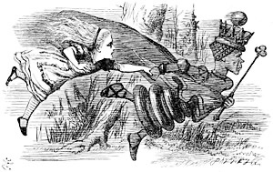
See the companion postGovernment Finance 102: Monetary Policy: The Red Queen’s Race for how the Fed has facilitated the creation of our large federal deficit. For many years, the Fed kept the fed funds rate close to zero; this meant the government could increase borrowing faster than interest expense. Almost free money.
You might want to pair this essay with the latest population and demographic projections (fewer people, more old people). See
If CBO trendlines were projected out to 2045, the national debt would be more than $70 trillion. U.S total population and the size of the labor force in 2045 is very likely to be less than now. Retired Americans will be a higher percent of the total population.
The CBO assumption that nothing will ever go wrong in the U.S. economy isn’t likely. To be fair, this restriction was put on the CBO by Congress.
Elsewhere in this blog, I argue that the main form of our economic competition, and geopolitical rivalry, with China will depend on our success in developing new technologies. See
If the United States maintains the current proposed tariffs averaging around 15-20% and because of current economic policies cannot compete with China in global markets, CBO and other economic projections are unrealistically optimistic.
For a list of all the posts on this blog, see
List of Posts by Topic
with links to all other essays. There are posts on the demographics of other countries and the world as a whole, the Beginning of the Industrial Revolution, American Economic History, and American History. Even posts on finance, business, and economics.
The Fed funds rate is the interest rate banks charge other banks that borrow their excess reserves. It is a very short-term (overnight) rate. An increase in the Fed funds rate increases the cost of capital of large banks (net borrowers) and puts pressure on these banks to raise their lending rates. A change in the rate also changes the rate charged by other sources of short-term funds.
The Fed funds rate is the most watched interest rate in the United States and probably the world. It is not set by supply and demand in financial markets. It is set (fixed) by the Federal Reserve Bank (the Fed), America’s central bank.
The Fed funds rate determines or heavily influences almost all other short-term interest rates in financial markets. It also indirectly influences many other longer term interest rates. It summarizes how the Fed views the economy and near-term changes. It is at the heart of monetary policy.
Nominal vs. real interest rates.
Nominal interest rates are the reported interest rates, also called current interest rates. Real interest rates are nominal rates minus some measure of inflation. Both nominal and real rates can be negative. For many years recently, nominal interest rates on many countries’ national debt have been negative. No longer. Although almost all countries have raised central bank rates, the inflation rate in the United States and many other countries was above almost all nominal interest rates, making real rates negative. This is no longer true in the U.S., as inflation has come down below the Fed funds rate but the Fed has not started to lower rates. (As of 7/24)
MONETARY POLICY
The Fed’s mandate is to make monetary policy. The objectives of monetary policy and the tools the Fed uses to implement policy have changed from the past.
In the past, the Fed’s main functions were to fight inflation by raising interest rates and slow down the growth rate of the money supply, and to fight recessions by lowering interest rates. The Fed could also be the “lender of last resort” to banks if the banking system got into serious trouble. Most of the time, however, the economy grew and the Fed had little to do. In the last few years, especially during Covid and after, the Fed has bought huge quantities of federal debt (Treasuries) to keep interest rates low. It is currently slowly selling off its inventory. It is uncertain if the Fed will continue to sell off Treasury inventory when it starts to lower interest rates.
Although never publicly stated, the Fed seems sensitive to supporting asset prices, particularly stock prices. Bond prices move inversely to interest rates. Rising interest rates lowers prices of existing bonds and raises the interest expense of new debt. The largest single borrower is the U.S. government.
With the deregulation and globalization of the banking system and the explosion of nonbank financing, the Fed has less direct control of the finance sector than in the past. But as long as the dollar is the international currency and non-bank financial institutions fund their operations by borrowing from banks, the Fed will have indirect influence on the rest of the financial markets.
The Fed funds rate is in the range of 5.25-5.50% while the inflation rate is under 3.0%. This has been the Fed funds rate since May, 2022. The Fed started reducing the Fed funds rate to 4.75-5.00% in September. If the inflation rate stays low, this will decrease both nominal and real rates of interest.
The recent history of Fed policy has been unusual. The Fed under Ben Bernanke and Tim Geithner and the Treasury under Henry Paulson were extremely aggressive during the 2008-09 financial crisis in containing the real threat of a total meltdown of the national and global financial system. They extended loans to and guaranteed debt of banks and non-bank corporations. They promoted shotgun marriages between banks, creating megabanks and accelerating the consolidation of the banking system. But their policies of historically low interest rates and purchasing of public debt continued long after the economy resumed growing. From 2008 to early 2022, the Fed funds rate has been below 1% in 12 out of the 14 years. This is extraordinary; the last time the Fed funds rate was below 1% was for a short time in 1958. And, during this recent past period, real interest rates were negative. The Fed obviously believed that a massive interest rate subsidy was necessary to get the U.S. economy out of the Covid-caused recession and for continue economic growth.
A major beneficiary of low interest rates has been the federal government. The government has been able to greatly increase the national debt with little increase in interest expense. Interest rates on government debt before the 2022 inflation, less than 1% on ten-year government bonds, were the lowest they’ve been since the end of World War II. But since 2022, interest expense on the national debt has been rising rapidly and will continue to rise unless there is a large decrease in government borrowing costs. This is unlikely.
Extremely low interest rates by themselves did not seem to have much of an impact on economic growth rates. But a combination of low interest rates and the corporate tax cuts of President Trump have helped to increase after-tax corporate profits. They have grown much faster than the economy and total income, reaching a record high as a percent of GDP. Over the last 40 years, stock prices have increased faster than wage income. No wonder families with financial assets have seen their incomes grow faster than families without financial assets.
While the Fed has increased the number of tools it is willing to use, it usually cannot prevent accelerating inflation or a recession. These are often caused by exogenous (outside) events the Fed has no control over. OPEC raising oil prices, Asian and Russian debt crises, Covid, Chinese lockdown policies, global supply-chain problems, war in Ukraine, Russia shutting off oil and gas supply to Europe, disruptions caused by effects of global warming. The Fed is judged on how quickly and effectively it reacts.
THE CORONAVIRUS AND MONETARY POLICY
The Federal government spent trillions of dollars to maintain total income, keep companies and state and local governments from going bankrupt, paying for emergency services and once again backstopping the entire financial system.
The government’s financial response to the coronavirus was unprecedented in peacetime. Starting with the 2008-10 playbook, the Fed and the Treasury, working together, came up with massive new programs to keep the economy from falling into a prolonged depression, buy time until the virus abated, and guaranteed virtually all debt in the country. In the first round, over $3 trillion will be spent on income maintenance. Congress added another $1.9 trillion in the first months of President Biden’s administration, which will be spent over the next decade.
All of the government income maintenance programs cost at least $300 billion a month, about equal to the fall in total income. This was extraordinary – a deep recession (fall in total output and rise in unemployment) without a decrease in total income. The economy recovered quickly. There were falling levels of unemployment already in 2021 and near record lows by the first half of 2022. Since then, the unemployment rate has remained low despite a continuous increase in the size of the labor force.
The lagged effect of earlier income maintenance programs plus the 2021 “stimulus” expenditures pushed total income above the long-term trend line, resulting in increases in total spending and falling unemployment rates. The inflation rate rose through 2021, reaching levels far above 2% before the Russian invasion of Ukraine and the resulting increases in energy prices. The Fed did not start increasing interest rates until the middle of 2022. But, to make up for a tardy start, it raised rates rapidly.
The Covid stimulus programs had another effect. Total household liquid financial savings went up by about $3 trillion, about equal to the cost of the programs. Add-on savings from higher income and a stock market boom has kept total liquid savings from declining very much, if at all. In other words, the net financial effect of Covid stimulus programs has been to increase public (federal government) debt offset by increased private (household) savings.
Assuming a 3% interest rate on the national debt, much of the increase in tax revenue since 2022 will go towards paying the increased interest expense on the national debt. Much of this has already occurred. Interest expense was around $450 billion a year in 2022; it is currently (2024) around $890 billion because of the increase in interest rates. By 2034, interest expense is projected by the CBO to be $1.7 trillion, about double the 2024 expense. By 2034, the increase in interest expense will be abut 60% of the increase in total expenditures minus the self-funding Social Security and Medicare programs. (BTW, the CBO projects that both Social Security and Medicare expenditures will increase about 5-6% a year. I find this hard to believe.)
For the details behind these projections, see The Congressional Budget Office. (Update as of June, 2024.), especially their Executive Summary.
How is the government paying for all this? Borrowing. Selling new debt to cover yearly deficits and rolling over existing debt at higher interest rates.
2020-2022
Much of the new debt created for the Covid programs was financed indirectly by the Fed, that is, the Fed created money to buy the same amount of debt. The Fed also underwrote the risks of virtually the entire debt market, even announcing it was willing to buy junk bonds. Much of the junk bond market consists of bonds issued by frackers who were in danger of going bankrupt because of low oil prices. The government would loan money and provide assistance (guarantee corporate debt) to companies in danger of going bankrupt.
2022 and 2023: FIGHTING INFLATION
All U.S. government fiscal and monetary programs in 2020 and 2021 were aimed at countering the sudden recession and economic dislocations caused by the Covid epidemic. But throughout 2021, the Fed was ignoring the financial effects of the stimulus programs financed by Fed’s buying of the rising national debt and massive expansion of the money supply.
The Fed has stated for a long time that it will tolerate an inflation rate of 2% but will be concerned if the inflation rate goes above 2%. The inflation rate started to go above 2% in March, 2021. It rose steadily to 7-9% by the end of 2021 (depending on which measurement was used). The unemployment rate fell rapidly, reaching 4% by the end of the year. The unemployment rate has been below 4% since 2022. This is close to what economists consider full employment. Until March, 2022, the Fed continued to purchase large amounts of U.S. government debt.
The $1.9 trillion stimulus program of March, 2021 was “a bridge too far.” A smaller program was probably needed to continue the recovery. The problem was the size. If you (or Fed economists) added the creation of new income to the trend in total income due to the rapid increase in employment and wage income, the total was greater than the amount of total income leading to full employment. That suggested that sometime in the foreseeable future (the Fed’s planning horizon), the inflation rate would go up, well past 2%.
Even with the inflation rate around 7% at the end of 2021, the Fed didn’t react. The Fed funds rate was still around zero. The inflation situation was made marginally worse by Russia’s invasion of Ukraine in March and the rise in energy prices (since reversed, at least the U.S. price of crude oil). Not until May, 2022, did the Fed start getting serious about raising the Fed funds rate and stop increasing its holdings of government debt. The Fed raised rates rapidly to make up for its delayed reaction to high inflation. They raised rates even while the inflation rate was coming down.
MONETARY POLICY AND MACROECONOMICS
The Fed made it clear they would keep the Fed funds rate high until the inflation rate would show a substantial downward trend towards 2%. Back to the old-time religion – fight inflation come hell or high water! Don’t support any aggressive fiscal policy to fight a possible recession that might result from rising interest rates. In fact, the Fed, to support higher Fed funds rates, has been selling its holdings of government securities to reduce the money supply. This risks the possibility of a recession before the inflation rate falls below 2%.
The Fed could get lucky. Many commodity prices are falling, which might counter some of the increased wage and salary costs. Shortages due to global supply chain dislocations started to clear up. Almost all large corporations are saying they are “increasing free cash flow,” a nice way of saying they are slashing costs. A recession might lead to a moderate increase in measured unemployment because the labor force is growing at a much slower rate than in the past. Fewer than expected new entrants. So small increases in the unemployment rate, as are now happening, do not seem to influence the Fed to lower the Fed funds rate.
If the price index as measured by some version of the CPI stops going up but stabilizes at the current high levels, the year over year inflation rate will go down. Why? Because the price level – the inflation rate – rose rapidly in the second half of 2021. The same current price level will be divided by increasingly higher past price levels, resulting in a lower yearly inflation rate.
Leads and lags again. Don’t “follow the data,” which is past news. Since there are lags in reporting economic data and the Fed has to look at trends and averages in the data, it will usually be behind the current and near future data. If there is large and rapid increase in the data, as recently, the Fed has to make up its delays in policy changes by large and rapid changes in instruments like the Fed funds rate. Anticipate the future and build in lags in the impact of policy changes. Like everyone else making financial decisions, the Fed should forecast the future and place its bets. As my old econ prof used to say – you puts down your money and you takes your chances.
The Fed should have anticipated that an aggressive monetary policy supporting massive fiscal stimulus to fight the disruptive recession caused by Covid could led to higher inflation rates if taken too far. As it did, the Fed should have started fighting the resulting inflation earlier, before it accelerated and raised inflation expectations. Large, delayed increases in the Fed funds rate chasing higher inflation rates now runs the risk of impacting the future economy as it enters a recession. To continue with cliches – the Fed gets the devil and the deep blue sea at the same time.
CONCLUDING REMARKS
There are indirect effects of the Fed’s monetary policies. Very low interest rates, money creation, bailouts to avoid company bankruptcies, and massive bond buying to avoid debt defaults all directly or indirectly helped stock prices. Asset prices increase while the real economy has falling inflation. But the 2021-22 inflation and rise in interest rates temporarily reversed asset price increases, especially stock prices. Since then, the stock market has had a strong boom, fueled by AI stocks (especially Nvidia) in addition to general rising corporate profits and speculation in crytocurrencies. The increased return on bonds does not seem to have diverted demand for stocks.
In short, the Fed bought massive amounts of private and public debt and paid for it by creating money. The federal yearly deficit is structural; unless there are radical changes in government spending and/or tax rates, the yearly deficit will continue and the national debt will increase.
This is short-run Keynesian economic policy on meth. Massive income maintenance through deficit spending. This is unlike government spending in the Great Depression, when some of the government spending led to public investment and new jobs – WPA, PWA, CCC, TVA, dams, rural electrification. The recent infrastructure bill provides potential tax subsidies to private investment in designated industries, particularly public investment, domestic chip production and renewable energy. Even before passage of the bill, large, global chip designers and manufacturers announced investment in new plants in the United States.
This is also Modern Monetary Theory on steroids – run large fiscal deficits and have the central bank (the Fed) create electronic money to buy the government debt. Keep interest rates low, preferably near zero, so the federal government can continue to run larger and larger deficits with small increases in the total interest expense on the national debt. The government has been doing this for years; only the high inflation rates forced the Fed (and financial markets) to increase interest rates.
There is research done by Carmen Reinhart, Vincent Reinhart, and Kenneth Rogoff that when government debt rises above 90% of GDP, economic growth slows down. Government debt held by the public is already above this ratio. The CBO projects the ratio will be 122% in 2034.
What if the causality is the other way? Or there are feedback effects? What if slowing economic growth and low rates of inflation mean a slowing growth rate in taxable income? In the “everybody wins” fantasy of democratic politics, it is difficult to control total spending or to refuse tax cuts or tax breaks. Rapidly rises expenditures for Social Security and Medicare because of an aging society is increasingly paid for out of general tax revenue. Payroll tax rates for Social Security and Medicare might not rise. When the Social Security Trust Fund goes to zero in the mid-2030s, about 20-25% of Social Security expenditures will come out of the general budget. This could add about $300 billion to yearly deficits.
Total tax revenue for the rest of the decade will only cover Social Security, Medicare, interest expense, government pensions and social welfare programs like Medicaid and food stamps. The rest of the budget – defense and discretionary spending – will be paid for out of borrowing. Borrowing more money is politically easier than “fiscal discipline.” Surprisingly, the CBO is projecting that short-term government borrowing rates on national debt will go down, but longer rates will stay about the same. This implies that average rates will decrease and the inverted yield curve will disappear.
All of these fiscal and monetary trends can go on for a long time but not forever. Japan has been doing this since the early 1990s, soaking up most of the country’s past savings to fight off a stagnant economy, deflationary pressures, an aging population, and lack of any structural reform. Japan has had very low rates of economic growth over the last 30 years; I doubt if the U.S. economy and society could tolerate very low growth rates over a long period of time.
The U.S. can continue running large budget deficits as long as the dollar is the international reserve currency, interest rates decline from current levels, and U.S. government debt is considered risk-free. Or if the growth rate of national debt is lower than the growth rate of nominal GDP. Currently, interest rates on the national debt are trending higher as the government rolls over the existing debt and attempts to attract buyers of the large amount of new debt.
In the past, conventional wisdom said that fiscal policy and monetary policy had contradictory goals. Fiscal policy was supposed to encourage and support economic growth and job creation. Deficits would increase if there were a recession or low economic growth. This was in the personal interest of elected officials. But too much stimulus or for too long could lead to higher rates of inflation. The Fed would then raise interest rates until inflation rates eventually came down. This would slow down spending and risk a recession. But over the last 30 years or so, the two institutions seem to be coordinating their policies. The government now has structural deficits rather than a counter business cycle (Keynesian) strategy. The Fed has a bias towards low (below market) interest rates, which also encourages borrowing and increased aggregate demand. Only if the inflation rate rises to a level that threatens growth will the Fed be aggressive in raising rates. So the CBO can project real growth, rising national debt, and falling government borrowing rates from the current levels. Even as the national debt/GDP ratio rises. Again, this might go on for a long time, but not forever.
This tutorial will look at financial markets and how they actually function.
There are two general theories about how financial markets work. The first is the Efficient Market Theory, which assumes all decision-makers are rational – they have access to information, can analyze it, and make investment decisions. Strangely, a major conclusion is that investors cannot predict stock price movements, which are random. The second is Behavioral Finance, which assumes that investors are irrational – they have a number of biases and are influenced by the markets’ past behavior.
Both theories based on this supposed distinction that “explain” financial price behavior are irrelevant.
What is left out of theoretical models of financial markets is how financial markets actually operate. Between buyers (investors) and sellers (including issuers of new securities), there are market makers like brokerage firms, managed funds, hedge funds and investment banks. It is in their interest to get investors to invest in financial assets rather than other types of assets, to trade often, to buy riskier securities and derivatives. All these strategies generate more revenue for them.
It is also in their interest to convince investors to pay large fees for supposedly superior information or analytical skill, that is, to ignore the Efficient Market Hypothesis. And investors, including large pension funds, often do.
The primary selling tools are financial information, analysis of the information, and forecasts. It is the self-interest of all market-makers to present biased information and optimistic forecasts. For market-makers, financial information and forecasts are marketing data.
What is financial information? First, the current earnings of companies. The problem is politely phrased “quality of earnings.” Earnings, and earnings per share (EPS), are routinely managed by corporate accountants to show steady or exponential earnings growth. This increases the share price as EPS goes up and, if earnings rise by a high or increasing percent every quarter, by increasing the price/earnings (P/E) ratio of the stock.
Since top management now receives much of its compensation from stock options and bonuses based on earnings growth, they have a personal reason to see that earnings are managed.
Even a casual reading of the financial press or case studies on corporate finance reveal the numerous ways reported earnings per share can be increased when there is no increase in operating earnings or even a decrease. The simplest way is to increase financial leverage. The current version is to borrow money to finance share buybacks. This increases earnings per share since there are fewer shares outstanding.
For a sample of corporate accounting frauds, see http://www.accounting-degree.org/scandals/. Also see the entertaining film The Smartest Guys in the Room for the massive accounting fraud that bankrupted Enron.
Then analysts who work for market-makers spin the earnings. They invent plausible reasons for the steady or accelerating increase in EPS and P/E ratios. Assuming these reasons will continue if not accelerate, they make optimistic forecasts of future earnings. Since the stock market is “forward-looking,” these biased forecasts are important pieces of “information” that investors use to make decisions. Analysts (and CNBC) become cheerleaders for the industries and companies they study, especially if they work for a financial institution that competes for investment banking business. Often analysts will hype a company that they privately know is a dog.
Analysts overwhelming issue buy or hold recommendations and very seldom issue sell recommendations.
The worse scenario for an investor is an industry with new technology. Analysts are free to make whatever predictions they want, no matter how improbable. A good story sells. In the decades I’ve followed the stock market, I’ve never heard an analyst tell the simple truth: Almost all the companies trying to develop a new technology will go bankrupt and it is impossible to tell which few will be big winners (if any). Think about the biotech, dotcom and “clean energy” booms. I think it is fair to include the clever innovations that made the subprime mortgage and derivative boom possible.
Investors are buying the future. Even stock index funds, which are weighted averages of the market value of the underlying stocks, go up mostly because of the more rapid than average increase in the hot stocks and hot industries.
This game comes to a temporary reversal when there is an “external shock” such as a recession. The phrase indicates important events than cannot be forecasted. Then there are the inevitable losses, “restatement of earnings,” “extraordinary losses” and “write-down of assets.” Hyped new technology companies go bankrupt. Hot stocks and industries driving the market get clobbered and indexes go down. Often a lot.
Besides reducing past earnings, companies will also take a “big bath” write-off of assets and anticipated future expenses. It is common practice to overestimate future expenses and losses. Then when actual expenses are incurred, they are smaller than announced and earnings are higher. This is one reason for the apparent paradox that a company’s stock price often goes up when the company announces a large loss and a large write-off of assets.
But memories are short, hope springs eternal and there is always a new story to tell – a new hot industry, new hot companies, especially if in a new technology. And the game moves to a different location.
The main point here is that even if investors “rationally” analyze the biased information and forecasts, their subsequent behavior will not be any different than “irrational” investors who follow trends created by the biases and asymmetries of the financial information.
UNDERPRICING RISK AND FAULTY MARKETS
An important part of the information used to make investment decisions is forecasts. Yet the analytical tools used to forecast, and also price financial instruments, are defective. They are mostly based on a normal distribution of price movements and related linear regression models. Normal distribution models underestimate the probability of a large downward movement in stock prices. The market has much more risk (volatility) than the models indicate. Some of the studies and statistics are summarized in Benoit Mandelbrot, The (Mis)Behavior of Markets. This conclusion has been popularized in the best-seller, Nassim Taleb’s Fooled by Randomness.
A recent example was the credit default swap market. The pricing of credit default swaps in the 2000s was based on a correlation model that assumed away the possibility of defaults! Since AIG thought there was no risk of actually paying off for defaults, it underpriced the credit swaps and could not afford to hedge its positions. The resulting defaults of derivatives and investment companies led to the bankruptcy of the largest insurance company in the world.
There are some markets that cannot be forecasted. The bond market is bigger than the stock market. Yet economists cannot forecast interest rates and thus the movement of bond prices. The mortgage market cannot be forecasted. The future cash flows of variable rate mortgages are highly uncertain and fixed rate mortgages can be refinanced. Thus the future cash flows of mortgage-backed securities cannot be forecasted. Uncertainty is compounded by leverage in buying mortgage-backed securities(MBSs), the creation of derivatives based on MBSs, and default risk.
INDEX FUNDS VERSUS MANAGED FUNDS AND PICKING STOCKS: INFORMATION AND IGNORANCE
Financial markets are information rich. According to economic theory, prices should reflect this information. The pricing mechanism should be very efficient, summarizing the analysis of the large amount of data. But most individual investors and many institutional investors such as pension fund trustees are totally ignorant of financial markets and incapable of interpreting and analyzing financial data. What to do?
1) Pay someone else to analyze data and pick stocks. (Managed funds)
2) Buy index funds and index ETFs.
An index fund like the S&P 500 ignores the problem of picking good stocks and buys the entire stock market. Stocks in the index are weighted by their total market value (in the jargon, called “market cap,” short for market capitalization). So the index buys 10 times as much of a stock with a market cap of $100 billion than another stock with a market cap of $10 billion. The index has to adjust the weights as the relative market caps change.
Indexes tend to be dominated by very large companies and rapidly growing technology companies with high and rising P/E ratios. Before the 2008-2009 crash, indexes were dominated by financial companies. Six of the top ten market cap companies in the S&P 500 are tech companies. Currently (2018), the eight companies in the world with the highest market cap are all information technology companies.
“Buying the market” (index funds) rather than individual stocks is a strategy for totally ignorant investors. Much of the increase in money going into the stock market after the 2008-2009 crash has gone into index funds and index ETFs. All that investors have to assume (believe) is that the real economy will grow, total profits and earnings per share (EPS) will thus increase, and that most if not all stock prices will rise as a consequence. Investors can ignore the competitive strategies and financial performance of individual companies, industry analysis, monetary and fiscal policies, and global and macroeconomic trends.
And total ignorance works. A great deal of statistical evidence indicates that index funds outperform over 90% of managed funds over long periods of time. They also have lower costs – no expensive analysis costs. Managed fund managers also tend to take greater risks and create leverage (invest with borrowed funds in additional to investors’ money) to offset higher costs and achieve higher rates of return than index funds. Because of greater leverage, greater risk, and high costs, managed funds tend to do poorly in stock market downturns. Many “blow up” (go out of business).
Index funds work because in the long run the economy does grow, total profits of public companies rise, and most stock prices go up. As more money goes into index funds, the funds must buy more of all of the stocks in the fund. The whole market goes up and the index funds prosper.
All of this also benefits managed funds. Experienced fund managers with access to all past and current financial and economic data, data and trend analysis programs, and proprietary models should be able to outperform the market in such an environment. But they do not. Why?
They are making decisions based on biased and misleading information.
There is a problem of too much information that is hard to analyze. For example, many companies no longer release an annual report. Instead, they send their stockholders (and analysts) their 10-k, which is the annual report they have to file with the government’s Securities and Exchange Commission (the SEC). These are incredibly detailed reports with small type that go on typically for 100-150 pages. Most of the content is unimportant or irrelevant. (This is the mushroom effect. How do you raise mushrooms?Keep them in the dark and pile manure on them.)
They tend to buy companies with rapidly rising sales and profits. These companies also have high and rising P/E ratios during the innovative, rapid growth phase, increasing the rise in the stock price. As these innovative companies mature, their growth slows down. Profit growth also slows down or stops. P/E ratios fall. The result is a drop in their stock price, often large, followed by mediocre stock performance. Many of these companies are attacked by smaller companies developing or using newer technology.
Companies like IBM, Microsoft, Intel, and Oracle were innovative growth companies, are now large and profitable, but have been lousy stock investments for a long time. The large percentage increase in their stock prices in 2017 and early 2018 looks similar to the large runup in their prices in 1999, just before the dotcom market crash of 2000-2002.
Professional investors cannot predict “phase transitions” in industry technology or organization, or in the underlying economy. Just as it is difficult to predict the winners developing a new technology, it is difficult to predict the losers they will replace. It is the winners, not the losers, that make it into the indexes.
Managed funds do a lot of trading – buying and selling stocks in their portfolio. They try to time their trades with major moves in the stock market. This is difficult to do. Very few investment professionals ever predict market downturns.
Some managed funds buy a subset of large, mature companies. A diversified portfolio of about 30 stocks reduces risk almost as much as a total market index. Their economic performance as a group will be about the same as the large, mature companies in the index funds. With about the same sales and profit growth over time, the subsets in the managed funds should have long-term stock price increases about the same as the market. But at a higher cost.
On average, about 60-70% of an individual stock’s price movement will be correlated to the price movement of the whole market. So, much of the movement of stocks in a managed funds will move with the market, especially a managed fund dominated by large companies with large market capitalization.
Some large cap companies are so diversified that they are a diversified portfolio in themselves. Johnson & Johnson could represent much of the pharmaceutical and health care industry. Parker Hannifin could be a proxy for investing in cyclical industrial companies. Companies like Google and Celgene buy or invest in new and small technology companies in their industries, almost like a venture capital company. Many large companies not only have a diversified business but are also multinational corporations, a proxy for investing outside the United States.
Some managed funds concentrate on innovative companies. The problem is that many new tech and startup companies fail; their stock prices will go to zero. Many did in the 2000-2002 dotcom market downturn. They took a lot of managed funds down with them.
As discussed throughout these tutorials, an important factor for the success of a startup is the drive, determination, focus, and strategy of the founders/entrepreneurs. It is hard for an outsider like an investment manager to evaluate the intelligence, dedication, and personality of the founders.
Outside analysts and investors do not have the key information they need to evaluate a company – the internal detailed proprietary knowledge responsible for the competitive advantage causing sales and profit growth.
Most stocks, including those of the large, mature companies that tend to dominate index funds tend to go up and down (are correlated) with the overall market. There may be individual exceptions because of company-specific events but as a group they heavily influence (account for) overall stock market changes. There is no need to try to pick individual stocks among this group.
Often, one sector drives the market – IT and Internet stocks in the 1990s, finance in the 2000s, and technology in the 2010s. It is hard to pick winners early and the timing of the downturn is also unpredictable. Index funds ride through the downturn and are there for the next upturn fueled by innovative companies in new sectors and industries.
There are internal dynamics of the stock market. Companies increase dividends, buy back their stock, and do mergers and acquisitions. All these moves can increase the price of an individual stock; collectively, they increase the value of the entire stock market. Index funds automatically benefit. Managed funds often do not.
Picking stocks to outperform the market critically depends on predicting growth rates in expected EPS for years into the future. Any forecast will be highly uncertain and subject to large errors.
In conclusion, the stock market is not a random walk (impossible to forecast) or the result of irrational, emotional behavior by investors and money managers. Professional money managers seldom “beat the market” because of uncertain forecasts, the domination of mature companies, the difficulty of outsiders to pick innovative winners, and incomplete and misleading data.
I recommend reading Burton Malkiel, A Random Walk Down Wall Street. Revised and Updated Edition, 2007. Professor Malkiel was associated with Vanguard for a long time. Earlier editions of this book were an argument for the index fund approach to investing made popular by Vanguard. This edition gives a more balanced approach than earlier editions.
INSIDER INFORMATION:PROFITING FROM ASYMMETRIC INFORMATION
Financial markets are rife with insider information. Inside information is a classic example of asymmetrical information, where insiders can profit at the benefit of investors not yet knowing the information. Sometimes insiders use their information and position to manipulate prices, such as the massive LIBOR price-fixing scandal.
Many foreign markets are insider markets, where locals can conspire to manipulate and fix prices, especially at the expense of foreign investors. This is similar to what U.S. markets were like before the reforms of the 1930s.
FINANCIAL MARKETS AND MORAL HAZARD
Conservatives argue that deregulation of financial markets leads to innovation and more efficient markets. The first part is true; many new financial instruments and new types of financial companies have been created. The implication of the second part is that because of more competition prices in financial markets quickly adjust to something approaching “fundamental value” or, in economic jargon, equilibrium. The basic problem is that the first effect works against the second effect.
The problem is moral hazard, an idea that says that individuals like managers and owners of financial institutions will take more risk if someone else (the U.S. government and taxpayers) pays the price of failure.
This happened in the savings and loan crisis of the late 1980s. The industry was deregulated so that S&L managers could make riskier loans at higher interest rates but deposits were still federally insured. So the more aggressive banks offered higher interest rates on deposits, took in a lot of money, and made a lot of high-risk bets, including illegal loans to insiders. They lost. Half of the S&Ls went bankrupt and it cost U.S. taxpayers over $130 billion in losses on bad loans.
Deposit insurance is one source of moral hazard. Another is that the two largest players in the mortgage market, Fannie Mae and Freddie Mac, had the implicit guarantee of the government. A third source is the “too big to fail” doctrine, already invoked in a big bank rescue in the 1980s. Combined with that is the idea of “systemic risk,” which implies that if a financial institution failed, even if it wasn’t a bank or “too big to fail,” it might set off a chain reaction that would threaten the collapse of the entire financial system. This is what happened with the failure of Long-Term Capital Management in 1998.
EXTREME RISK AND TOO BIG TO FAIL:LONG-TERM CAPITAL MANAGEMENT (LTCM)
In the 1990s, the company with the most sophisticated models and trading strategies was Long-Term Capital Management. Its partners included the former head of bond trading at Solomon and two Nobel Prize winners for their work in financial models (Myron Scholes and Robert Merton). Its strategy was based on reversion to the mean of the difference in the prices of a large number of supposedly unrelated financial instruments, another correlation model. But in the global financial crisis environment of 1998, the difference in prices moved in the opposite direction of historical behavior partly because of a “run to safety” in buying U.S. Treasuries. Spreads between Treasuries and other instruments increased instead of the expected decrease. This, plus enormous leverage based on underestimating risk, led to a massive bankruptcy. Only a huge infusion of capital from other firms, made under pressure from the Fed, averted a financial crisis.
LTCM was a hedge fund so the government had no legal obligation to intervene. It also wasn’t that large in terms of capital invested. But it was very highly leveraged, meaning it had borrowed a huge amount of money (about 30 times its invested capital) and had over $100 billion of assets and liabilities on its balance sheet. If it failed, its lenders and counterparties to financial contracts would take a huge hit; it was believed that some credit markets might even freeze up (become illiquid). The Fed decided that this was too big a risk to take and forced nine major banks to chip in over $3 billion to carry the assets. LTCM was liquidated and its positions were eventually sold. But it established a precedent that a threat to financial markets, not necessarily the size of the company or the legal obligation of the government, might be a reason for the government to bailout a company. And the threat to financial markets was rapidly increasing as all large financial institutions increased their leverage in the 1990s and 2000s, many to the 30-1 ratio of LTCM. They were using borrowed funds to buy and trade inherently risky mortgage-based bonds and derivatives.
BIASED INFORMATION, FRAUD, EXTREME RISK, AND TOO BIG TO FAIL:THE SUBPRIME MORTGAGE MARKET CRASH OF 2007-2009
After the Dotcom market bust of 2000-2002, the market continued upward, fueled by tremendous gains in the financial markets. Financial firms had found a great new business – securitizing mortgages and other debt instruments and selling bonds and other derivatives based on the cash flow of the underlying assets. At the foundation of this was a huge increase in subprime mortgages and mortgage refinancing. Many of the subprime mortgages were blatantly fraudulent or certain to go into default. But banks and other financial institutions were able to sell pyramids of derivatives many times greater, and more profitable, than the original issuance of mortgages. These markets were totally unregulated. (To understand how all this happened, see the movie The Big Short and read Explaining Derivatives – An Analogy after this essay.)
The subprime mortgage business was a con game from the start. Mortgage brokers and loan officers at sketchy banks used deceptive and often fraudulent methods to originate subprime loans. Mortgage and mortgage-baked securities (MBSs) risk analysts at some banks and investment banks, the credit rating agencies, and Fannie Mae knew that there would be a high rate of default after the low “teaser” rates ran out. In loftier language, Alan Greenspan warned in 1994 that there was a good possibility of a housing bubble and massive defaults of mortgages.
The problem was how to sell these “junk” mortgages. In a rational market, investors in subprime mortgages and their MBSs should have received high rates of return to balance the high risks of default. Not to be. If banks kept the mortgages, they could be financed by low-cost short-term borrowing. Why low cost? Because throughout most of the 2000s, the Fed kept short-term interest rates low. The prime rate was below 2% for three years.
But banks sold most of subprime mortgages to other financial institutions that would securitize the mortgages into bonds backed by the monthly payments of the mortgage holders. The bonds should have paid a high rate of return. But they didn’t. The reason was that these mortgages and their derivatives were laundered. The financial industry, with the connivance of credit rating agencies that were paid by the banks, turned bundles of high-risk mortgages into bundles of investment-grade (low-risk) bonds. Then the riskier parts of these bundles were turned into new derivatives that were also rated as investment grade. By labeling these securities as investment grade, this greatly increased the pool of potential institutional buyers such as pension funds. Mortgage origination fees, underwriting fees, selling fees and trading commissions were enormous.
But who bought these instruments? At the height of the subprime boom, large purchasers were Fannie Mae and Freddie Mac. In the past, both companies would have automatically rejected subprime mortgages. They didn’t even have models to evaluate these types of mortgages. As companies with de facto government guarantees, they were obligated to only buy and securitize high quality, low-risk mortgages. But under political and industry pressure, and loss of market share, they became major buyers of subprimes and sold mortgage-backed bonds at rates slightly higher than U.S. government bonds. Massive defaults led to the bankruptcy of both companies, which were taken over by the federal government. For political reasons, most of the losses were not borne by the bondholders such as the Chinese government but by U.S. taxpayers.
So the consequence of deregulation was not diversifying risk and self-equilibrating financial markets but accelerating systemic risk underwritten by moral hazard. How could it be otherwise? Selling greater volumes of increasingly riskier assets meant huge increases in salaries and bonuses. What did mortgage originators and managers of banks, investment banks and hedge funds care if they were creating higher levels of risk that could bring down their companies or the entire financial system? Increased leverage meant increased profits and increased bonuses. Fraud was rampant. Regulators were either clueless (SEC) or ignored their feelings that a crash was coming (Greenspan). Most deals were private so that even the hope of “free market discipline” was missing. Best of all, there were huge pools of funds run by unsophisticated trustees (asymmetric information) to finance the whole thing. Wall Street’s attitude was nicely summarized in a line from the movie The Magnificent Seven, “If God didn’t want them sheared, He wouldn’t have made them sheep.”
Will it happen again? Of course. The financial reform bill is a joke, nothing more than a political CYA crafted by the same politicians that helped create the mess. But the Congressional hearings were good theater as every member of Congress repeated a variation of the cynical line from the movie Casablanca, “I am shocked, shocked, to find out that gambling is going on in here!”
As part of its attempt to save the financial industry from imploding, the government brokered a number of “shotgun” mergers between large financial institutions. A small number of banks are now much larger than before the bailouts. They really are “too big to fail.” They are more dominant, gaining market share. They are also closely tied to the large hedge funds and private equity firms, which gives these private, unregulated companies some government protection. And, in a delicious irony, Goldman Sachs, a major private derivatives and trading investment bank, has applied to become a commercial bank so that FDIC can protect some of their creditors. The idea that American taxpayers are providing insurance to Goldman Sachs’ creditors, which include hedge funds, is moral hazard with a vengeance.
Government bailouts went way beyond the usual targets, to include insurance companies, General Motors’ and Chrysler’s financial arms, and GE Capital. There is delicious irony in the bailout of GE Capital. GE Capital is part of General Electric (GE), one of the largest corporations in the world. For many years, GE has paid no U.S. corporate income tax.
A last, major example of moral hazard. Public and private pension funds have made risky investments and lost. So what? The publicpension funds must have a certain level of assets in the future. So future taxpayers will pay more in taxes and receive fewer services. And $60 billion of unfunded liabilities in private pension funds are guaranteed by the government.
Large financial firms can expect public bailouts and subsidies when they “blow-up” but investors cannot. So financial firms can take excessive risks with investors’ money to earn large fees. It is only when they start to believe their own propaganda that the financial instruments they sell are really not as risky as they are, and begin holding the securities in their own portfolios, that financial institutions risk bankruptcy.
What this means is that in the future just about any company remotely related to finance can expect a bailout. There are no market restraints on risk left. The U.S. government is now underwriting the entire financial industry, no matter how reckless. And every risk-taking gunslinger in the future knows it.
CONCLUSIONS
Analytical tools and analysts are biased producing biased information and forecasts.
Statistical models underestimate risk. Risk is underpriced and uncertainty cannot be modeled. Combined with the upward bias in public information, this creates higher percent growth of financial prices in “normal” times followed by periodic “blow-ups” in financial markets.
Moral hazard allows investment managers to take great risks since they know that the government or taxpayers will underwrite large losses. The information and knowledge that most professionals possess does not give them an advantage over the total ignorance of investing in passive index funds. They cannot “beat the market.”
===============================================
EXPLAINING DERIVATIVES – AN ANALOGY
You go around to farmers with cows. You buy all the cows and pay the farmers a small fee to milk the cows and sell the milk. You pay for the cows with ass(et)-backed securities called MBSs (Milked Bovine Securities) that you tell investors are udderly safe. But some of the cows don’t give enough milk (cow flow problem) or give no milk at all. You take some of the asset-backed securities, say they’re backed by the subprime cows, and use them as collateral to sell another set of securities called CMOs (Cow Milk Obligations). Then you buy CDSs (Cow Dried-up Swaps) from AIG (Angus Insurance Company) to insure the CMOs when the cows stopped giving milk. If you work it right, you collect more on the CDSs than you pay out to retire the CMOs. The money you get from selling the dead cows go to pay the CLOs (cow leather obligations).
You could also sell CDOs (cow dung obligations) that depend on how much cow dung is produced. This is a typical Wall Street product – turning shit into gold.
INTRODUCTION: SIMILARITIES AND DIFFERENCES BETWEEN 1929 AND 2020
Gamestop! Short squeeze! Bitcoin! Options! IPOs! SPACs! Hydrogen trucks! Tesla up 800%! Market valuations in bubble territory. And my favorite “blue sky” stock – Virgin Galactic.
At first sight, there was nothing in 1928-1929 similar to the impact of Covid-19 on the economy. Actually, there was. In 1927, Ford closed down his entire company to retool for a new line of cars. 70,000 Ford employees were thrown out of work; many more at suppliers also lost their jobs. But everyone knew that Ford would start up production again.
Ford began production in 1928; 1929 was a record year for auto production. But in late summer and early fall, inventories began to build up.
Both periods were preceded by speculation in real estate. Both ended badly, closing off an alternative area of speculation.
Both periods (1920s and 2010s) saw an increase in income inequality. Large parts of the labor force, particularly farmers in the 1920s, saw stagnant or falling real income.
The assumption of endless growth based on new products, new forms of energy and mass production provided the foundation for the speculation in 1928 and 1929. Over the last 10 years, investors have believed there will be endless growth based on the development of new information technologies combined with the commercialization of an explosion of new knowledge, in biotechnology for example.
The long bull market starting in 2009 was accelerating in late 2019 and early 2020, similar to the long bull market of the 1920s. Then the virus hit, sending the economy into a deep recession. But unlike the Great Depression, the federal government stepped in with massive income maintenance programs. Despite high unemployment in 2020, real disposable income and consumer spending rose. Savings also rose, some of which found its way into stocks. As vaccines became available, it was assumed that economic growth, fueled by innovation and low interest rates, would continue.
One similarity was a part of the Fed, the New York office, reacted quickly to the 1929 crash. It lowered interest rates and made substantial sums available to the banking system to support the stock market. But it was a one-off; other regional Feds refused to provide liquidity to the system and the Fed governing board in Washington seemed willing to let the entire financial system go to hell.
In 1929, high-tech companies like RCA and growth companies with new products and services such as the electric utilities, were especially hard hit. Unlike the beginning of the Great Depression in 1929, the impact of Covid-19 led to massive changes in behavior that benefitted information-based companies. A handful of very large companies already dominated the market indexes; they would drive the indexes higher. Other companies such as Zoom and Teledoc saw a huge increase in demand. Media concentration on the race to develop a vaccine focused attention on small biotech companies developing new drugs and health care systems. All of this drove the stock market higher in the face of a sharp recession.
The economic decline stage of the Great Depression lasted for almost four years. The Covid recession was sudden and sharp. With the development and production of vaccines, it has an endpoint in the middle of 2021. And, learning from the “malign neglect” of the Hoover administration, the federal government, as in 2008, reacted quickly with massive income maintenance and aggressive monetary programs to limit the economic damage.
The rapid development of vaccines convinced investors that the economy would return to normal growth during 2021. Investors also believed that the subset of high-growth technology companies would continue their superior performance into the foreseeable future. All this sustained high stock market growth rates into early 2021 and beyond.
Most of the stocks with the highest percent gains in 2020, gains of 3-10 times for the year, are equities of companies that were losing money. Most have innovative, even disruptive, technology that would make them attractive parts of a long-term growth stock portfolio. But because of large R&D expenses, long and expensive drug trials, upfront capacity growth expenses, they would lose money for the foreseeable future. But large stock price increases in 2020 have already priced in spectacular long-run success. The best-case scenario is that their stock prices will not continue to rise. Many of the companies will fail. But the market as a whole will probably not collapse as in 1929-30.
PSYCHOLOGY OF 1928-29 AND 2020-2021 ARE SIMILAR (SO FAR)
In both periods, negative economic data and bear market sentiment were ignored. There were scattered indications in the late summer and early fall of 1929 that the economy might be entering a recession or at least had stopped growing. But almost no one paid attention. Anyone expressing bearish sentiments in 1929 was roundly denounced as a party pooper. Even un-American.
While there are now a few bearish voices, they are drowned out by the steady optimistic drumbeat of media commentators, brokerage and investment bank projections, and social-media driven popular culture. New investors believe the title of the most famous article written about the stock market in 1929 – Everyone Ought to Be Rich.
A few large investors were getting nervous or paying attention to the economic news in 1929. Jesse Livermore, maybe the most famous big-time speculator on Wall Street. J. P. Morgan partners; while they were putting out optimistic press releases and interviews, many were personally selling stock.
In both periods, there was a big increase in small individual (“retail”) investors (speculators). Estimates of new investors during 2020-early 2021 are as high as 10 million. As in 1928-29, these new investors expect big gains in a short period of time. In both periods, there was a large increase in trading volume, compounded in 2020-2021 by a huge increase in options trading. Risk was ignored. Speculations were leveraged; options in the current period played a similar role as margin accounts (put up 10%, borrow the rest to buy stocks) did in the earlier period.
In both periods, stock market speculation became a part of the popular culture. It seemed everyone was talking about the stock market, in private conversations and mass media. Investment decisions were based on rumor and gossip that went viral on the Internet.
But it wasn’t just the extreme examples. The whole market was in bubble territory. In early 2021, market indexes were at historically high levels compared to earnings (P/E and other ratios), even assuming a complete recovery of total sales and earnings over the next 12 months.
In 2020, a small number of companies benefitted from the changes caused by the virus. They dominated the indexes and accounted for much of the market rise. For example, about ten huge technology companies accounted for about 25% of the S&P 500 and most of the increase. Large parts of the economy, like farming in the 1920s, were hurt.
PSYCHOLOGY OF SPECULATORS
Why did the stock market “crash” in October and November of 1929?
The stock market peaked on September 3, 1929. It then drifted slightly lower for seven weeks. But speculators were expecting large gains in a short period of time. Many had margined accounts, paying interest on broker loans. Their patience ran out and some began selling in late October. Volume, already at record levels, rose even higher. Sellers overwhelmed buyers, including professional attempts to “support the market.”
Many middle-class families, the source of much of the new money in stocks, were also leveraged in their finances. The 1920s saw large increases in mortgages and consumer credit to buy new products such as cars and radios (which could cost as much as a new car). Farmers, collectively experiencing declining income in the 1920s, were saddled with long-term debt used to buy land and equipment before and during World War I. Middle-class families with assets in 2021 held most of them in the form of illiquid assets such as home ownership (with mortgages) and retirement accounts.
Many investors were sitting on unrealized (paper) gains in October, 1929. But the market has stopped going up. This may have indicated that the supply of new investors (greater fools) was not increasing. I expect something similar to happen later in 2021.
WHAT HAPPENS NEXT?
In early 1930, the stock market had a partial recovery. But the economy was in a recession. The recession got worse every month. In April, the stock market turned down; it would not start to recover until 1932.
Stock market investors are assuming that the economy will grow in 2021 and 2022. Even if true, real economic growth could be low. Lowered expectations of corporate sales and earnings growth, especially of large growth stocks and beneficiaries of the forced change in behavior in 2020 – 2021, could lead to a market correction.
The massive federal “stimulus” programs have done nothing to stimulate (increase) long-term economic growth. No increase in public infrastructure investment. No increase in government-funded R&D outside of Covid-19 vaccine development. No increase in government programs to reduce and reverse climate change. Because so much was borrowed during this crisis (over $4 trillion), it may be difficult for the federal government to borrow to adequately fund these programs in the future.
Even without any new government programs, the federal government will be running annual deficits of $1-$2 trillion a year. Unlike Japan, where large annual deficits are necessary to counter deflationary and recession tendencies, large deficits in the U.S. could lead to higher inflation rates. That would lead to higher nominal interest rates. The Fed would find it very difficult to keep short-term rates near zero. Every one percent increase in interest rates would add over $200 billion a year to the deficit.
Market indexes are already higher than the prior all-time high in February, 2020. Valuations (market P/E ratios) then were already at historically high levels. Even if corporate earnings and earnings per share reach 2019 levels over the next 12 months, they are being valued at higher, near-record historical levels.
The forecast here is that sometime in the first half of 2021, there will be a market correction. The proposed “stimulus” program will get the economy through the next 4-6 months as the adult population become immunized. It will be the last large such program, although the federal government will still have a large structural annual deficit. After adjustments in the service sectors of the economy, countered by much slower growth in the sectors and companies that benefitted from the adjustments during the epidemic, the economy will experience slower than historical growth. Growth will be concentrated in high tech, innovative sectors and companies. Interest rates outside of the short-term, low-risk debt will rise.
AN ALTERNATIVE SCENARIO
The main similarity between the two speculative periods is the increasingly speculative behavior of investors, especially the large number of new investors. Investors expect larger returns in shorter periods of time, ignoring the underlying fundamentals. Both periods became “momentum” markets.
A market correction in this environment, like in 1929, could happen for no apparent reason, no large “external” shock or internal surprise like a fall in earnings. Most likely, it might occur because of a fall in expectations.
Imagine, for example, that most adults who want the vaccine have received it by early summer. The economy returns to its economic growth path. Earnings of public corporations in 2021 accelerate and quickly return to 2019 levels; projections of 2022 earnings reflect historical growth. The bull market that began in 2009 continues.
But the market has already “baked in” high earnings growth in 2021 and 2022. Imagine a different scenario. Most of the proposed “stimulus” spending other than unemployment benefits is spent. The tremendous support for total disposable income and consumer spending stops. Despite widespread vaccine use, the virus continues at a lower level. The economy does not revive at expected high levels as there is still some hesitation to return to prior levels of demand for recreation, entertainment, leisure and travel. Many companies that benefitted from the “lockdown” find their sales and earnings stop growing, or even fall. Their stock prices fall. Other companies build on their experience during the virus to continue to reorganize their companies to cut costs and increase productivity by reducing overhead costs of offices and travel, and reducing employment by accelerating the substitution of software and automation for employees.
The increase in disposable income and consumer spending from increased employment does not make up for the loss of “stimulus” income. Projections become more uncertain.
I have no idea exactly when a market correction will occur, just as no one had any idea the market would fall in October, 1929. But I think it is most likely to happen sometime in the period of late May to mid-July. By late May, it may seem more probable the economy is not going to recover as vigorously as expected. Mid-July is when the first of the second quarter earnings are reported. Since the market anticipates change, especially short-run change in this environment, I would guess the correction would be more likely in the beginning of this period.
HOW LARGE A CORRECTION?
It is possible that the stock market could fall at the same time the economy is expanding, assuming the expansion and earnings growth are less than currently forecasted.
So, assume it is a typical market correction of a bull market. Maybe around 20%. If the S&P 500 had reached 4,000 or somewhat above, a 20% correction would bring the index back to its previous high of around 3,400 reached in February, 2020. Market valuations would still be at historical highs; the market could fall further.
What does this mean for individual stocks? Since the indexes are dominated by the large growth companies, this implies that as a group their stock prices will fall an average of 20%. But much of the rest of the last year’s tremendous stock market growth was caused by large percent increases in the prices of smaller growth companies. Many are technology companies that are losing money, especially small biotech companies. Many have doubled or tripled (or much more) since last March. There are no earnings or dividend floors under these stock prices. They could, on average, fall by two or three times more than the market – 40%-60%.
To the extent that travel and leisure stock prices had already recovered in anticipation of a return to pre-Covid behavior, these stock prices will also probably fall.
CONCLUSION
Current market multiples assume historically high economic growth rates in sales and earnings. It is more likely that for a variety of reasons, intermediate and long-term growth rates may be historically low. A reduction in growth rate expectations could lead to a market correction.
As in 1929, a change in expectations, even if not caused by any major expected change in the economy, could precipitate a market correction. It is a change in the expectations of some investors, in both cases expecting large returns in short period of time, that cause market corrections.
It is a cliché of investing that stock prices, and the market as a whole, are determined by the conflict between greed and fear. In a long bull market that has entered bubble levels of valuation, the conflict is between momentum based on optimistic assumptions and projections, and doubt (increased uncertainty about the projections). A market correction occurs when doubt increases and more investors decide to reduce risk or realize paper gains by selling growth stocks, hedging, or moving to a more conservative portfolio (so-called value investing).